
2.1) Market
A market is a place where buyers and sellers exchange goods and services. Eg- Stock markets, local markets like vegetable market, oil and labour market.
Types of Markets
Competitive markets are those markets which comprise a large number of buyers and no individual has the control over the price. Price is determined by forces of Demand and Supply.
2.2) Demand
Law of Demand and Demand Curve
Demand is a quantity of a commodity which a consumer wishes to purchase at a given level of price and during a specified period of time.
Concept of Effective Demand
It refers to consumers’ willingness and capacity to purchase goods at various prices supported by their ability to pay.
Law of Demand
- As price increases, Demand decreases
- As prices decrease, Demand Increases
Demand Schedule for Apples
Let us understand the concept of law of demand with the help of an example say Apples:
Price per kg | Qty. Of Apples demanded |
10 | 50 |
8 | 60 |
6 | 70 |
4 | 80 |
2 | 90 |
As we can see from the table as the price of the apple is reducing the quantity demanded for the apples increases. This is clearly verifying the Law of Demand. Price and quantity demanded are inversely correlated.
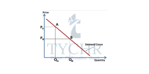
Demand Curve
As we can see in fig 2.3 as the price drops from PA to PB, the quantity demanded increases from QA to QB.
2.3) Why the Demand Curve slopes downwards
Marginal Benefit Theory
It is a maximum amount a consumer is willing to pay for an additional goods or services. It is the additional satisfaction or utility that the consumer receives when the additional goods are purchased.
Note: The marginal benefit for a consumer tends to decrease as consumption increases. That is why the Demand Curve slopes downwards.
Eg- Imagine you buy an ice cream which provides you with certain benefits. You want to buy one more, so you buy a second ice cream but the benefit derived from the 1st ice cream is more than the 2nd one. You enjoyed the 1st ice cream more in comparison to the 2nd one.
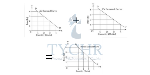
2.4) Individual Demand to Market Demand
Market Demand is the sum of the individual demand for a product from buyers in the market
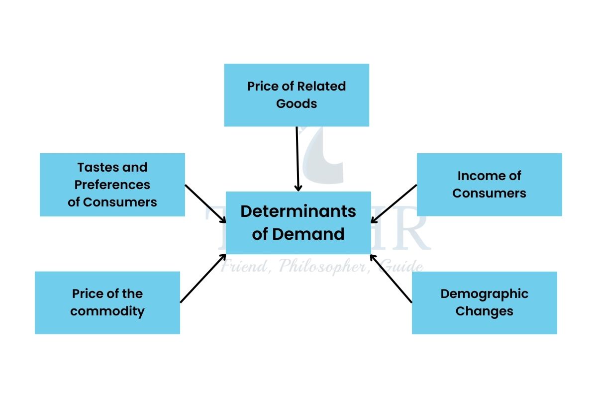
2.5) Shift of Demand Curve due to Non price determinants
Other than price, the other factors which affect the demand of a commodity are known as non-price determinants. These were the variables in Law of Demand which were assumed to be unchanged by use of the Ceteris Paribus assumption.
2.6) Shift of Demand Curve
Shift in Demand curve is due to non price determinants, price being constant.
Rightward shift in Demand Curve = Increase in Demand
Leftward shift in Demand Curve = Decrease in Demand
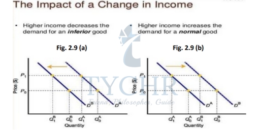
2.7) Income of Consumer
Impact on Demand Curve
In fig 2.9 (a), with the change in the income of the consumer, the demand curve shifts from DA to DB. DB<DA. Similarly in fig 2.9 (b), with the change in income, the demand curve shifts from DA to DB. DB>DA.
Price of related goods
To Sum-up:
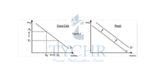
SUBSTITUTE GOODS
If Price of a good INCREASES, Demand for its substitute INCREASES.
COMPLEMENTARY GOODS
If Price of a good DECREASES, Demand for its substitute INCREASES.
Demand Curve of Substitute Good
Demand Curve of Complimentary Goods
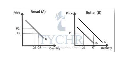
in the above fig, when the price of bread is increasing from P1 to P2, the demand for its
complementary good decreases from D1 to D2.
Tastes and Preferences
Favorable tastes and preferences results in increase in demand and vice-versa.
Demographic conditions
If the number of buyers are more the demand curve shifts right i.e. increases and vice versa.
2.8) Movement along a Demand Curve
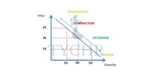
In the above figure, when the price increases from Pe to P1, the quantity demanded
decreases from Qe to Q1. This is called contraction of demand. Similarly, when price
reduced from Pe to P2, the quantity demanded increases from Qe to Q2. This is called extension of demand.
What is Supply ?
The Supply of an Individual firm indicates the various quantities of a good (or service) a firm is willing and able to produce and supply to the market for sale at different possible prices during a particular time period, ceteris paribus.
Law of Supply
According to the law of supply, the higher the price, the larger the quantity produced.
Supply schedule and curve
Let us understand supply with the help of an example of rice.
Price per kg | Qty. Of Apples demanded |
10 | 50 |
8 | 60 |
6 | 70 |
4 | 80 |
2 | 90 |
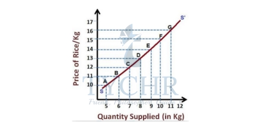
As we can see from the above figure, as the price of rice increases the supply is also increasing.
Market Supply
It is the total quantity of a good or service that all manufacturers are willing to sell for a certain price over a certain time frame.
Why does the supply curve slopes upwards?
A company has an incentive to produce more goods and vice versa because higher prices mean higher profits. As a result, there is a positive relationship between supply and price.
The Vertical Supply Curve
vertical Supply Curve = when the quantity of a good that is available cannot change, regardless of price.
Shift of Supply curve due to non-price determinants
2.10) The non-price determinants include the following:
Cost of factor of production:
Higher resource cost means lower quantity supplied.
Price of Related goods/ Joint Supply:
The production of goods derived from a single product is referred to as joint supply. Butter and skimmed milk, for instance, are made from sole milk. This indicates that an increase in the quantity supplied of one product will result from an increase in the price of another product.
Taxes:
Higher taxes imposed imply lower quantity supplied and vice-versa.
Subsidies:
It is a payment made by the government to the company to boost production. The supply will be greater the higher the subsidy.
Technology:
Improved technology means higher quantity supplied.
Number of firms:
Higher the no. of firms, higher is the quantity supplied.
Expectations:
If a firm expects the price of a product to rise, it implies lesser quantity supplied at present.
Sudden unpredictable events:
Natural catastrophes like earthquakes, war, floods, etc. affects supply.
Decrease in supply will move the supply curve upwards and Increase in supply will move the supply curve downwards.
2.11) Movement along the Supply Curve
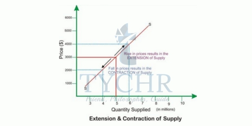
It happens because of the change in prices of the commodity, keeping other factors constant.
Market Equilibrium: Demand and Supply
Market Equilibrium is a state in which market demand is equal to market supply. There is no excess demand and supply in the market.
Equilibrium price and Quantity:
The equilibrium price is the price at which the quantity demanded and quantity supplied are equal.
The quantity demanded and supplied at an equilibrium price is known as equilibrium quantity.
Note:
Excess Demand-
It is the condition in which at any price demand> Supply
Excess supply-
It is the condition in which at any price supply is less than demand
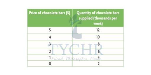
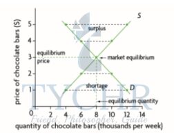
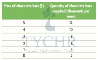
In the above fig. market equilibrium is at 8000 bars where supply= demand. At a higher price say at 4$ Qty supplied(10,000 bars)> Qty demanded(6000 bars). There is an excess supply of 4000 bars. With unsold output of 4000 bars, the firm will reduce the price, thus resulting in decreased supply which will further start increasing the demand and reach the point where qty demanded=qty supplied.In case of excess demand, say for eg at price 1$, Qty demanded=12000 bars and qty supplied= 4000 bars. There is excess demand of (12000-4000) 8000 bars, as a result, price increase which inturn increases increases supply and the quantity demanded begins to fall and this happens till the point where qty supplied= qty demanded.
2.12) Changes in Market equilibrium
Due to non price determinants, the demand and supply curve may shift leftwards or rightwards as the case may be, causing a state of disequilibrium.How is the equilibrium achieved in the following cases, it is discussed below:
Case 1: Demand increases
As demand increases, price also increases due to excess demand in the market from P1 to P2.As prices increases, supply will also increase from Q1 to Q2.
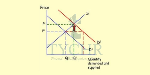
This will result in decreasing the demand, this happens till the new equilibrium point is reached.
Case 2: Demand decreases
As demand decreases, the price also decreases due to excess supply in the market from P1 to P2.
As price falls, the supply will also start falling from Q1 to Q2.
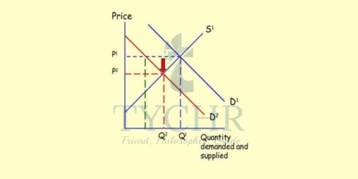
And in return the demand will start increasing. This continues till the new equilibrium point is reached.
Case 3: Supply increases
As supply increases, the prices will fall due to excess supply in the market from OP to OP1.
When a price falls, quantity demanded increases from OQ to OQ1.
Qty supplied starts decreasing till the new equilibrium point is reached.
Case 4: Supply Decreases
As supply decreases, a price increases due to excess demand in the market from OP to OP2.
As price increases, qty demand falls from OQ to OQ2.
This happens till the new equilibrium point is reached.
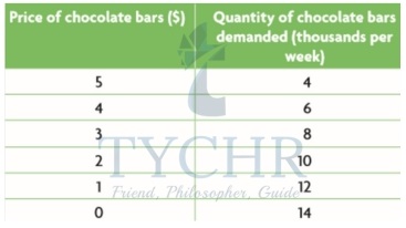
Linear Demand Function
Let us understand this with the help of an example. From the above equation we can draw a schedule and a demand curve.Eg: let us say demand function, Qd= 14-2P
Simply by putting different values of P we can obtain different quantities.
If we plot the above table on the graph, we can derive a demand curve.
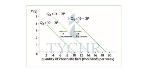
Change in parameter ‘a’ shifts the demand curve
In the above fig. a new demand function is obtained i.e. Qd=10a-2P, due to change in the value of ‘a’ which may be due to a non price determinant which has shifted demand curve to the left. Similarly, in demand function Qd=19-2P, again due to change in non-price determinant, the demand curve has shifted to the right.
Changes in parameter ‘b’ and the steepness of the demand curve
Slope is defined as the change in the dependent variable divided by the change in independent variable between two points. Eg- In the above equation, Qd = 14-2P, the slope is -2.Note: The greater the absolute value of the slope, the flatter the demand curve.
Linear Supply Function
From the above equation, we can draw a table and a supply curve; by substituting different values of ‘P’ we can get the quantity supplied.
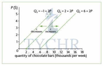
Change in parameter ‘c’ shifts the supply curve
Parameter ‘c’ is a non price determinant of supply. A change in the value of ‘c’ causes a left handed or right handed shift of the supply curve, as seen in the figure above.
Changes in parameter ‘d’ and steepness of the supply curve
Note: The greater the value of the slope, the flatter the curve.
2.21 Price mechanism
Price mechanism is the mechanism in which prices play a key role in directing the activities of producers, consumers and resources suppliers.
There are two important elements of price mechanism
(1) Prices
(2) Markets
The role of price mechanism in resource allocation:
Resource allocation: Scarcity, choice and opportunity cost.
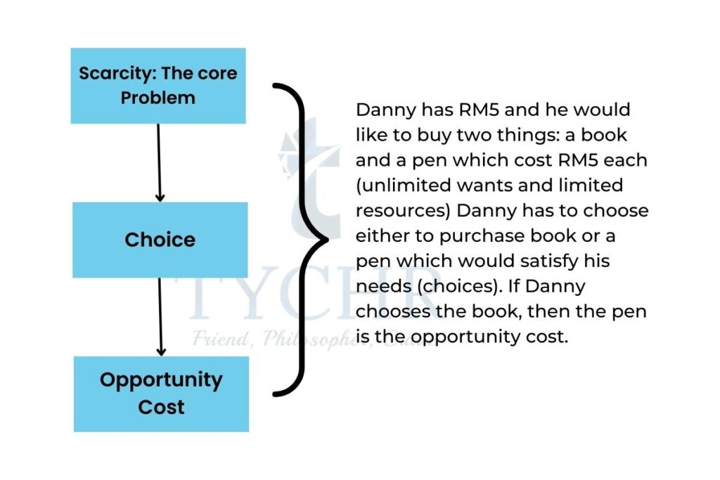
The above figure relates to the problem of resource allocation due to the scarcity of resources.
2.13) Resource allocation: Prices as signals and incentives.
Market mechanism working through prices is known as the invisible hand of the market.
How are Prices set in a Free Market?
Adam Smith- wrote the book Wealth of Nations
— Invisible hand
1. Producers will make what is most profitable
2. Consumers have incentive to buy goods at the lowest cost
3. These must be allowed to work itself out. There is an invisible hand controlling thing.
It works through 2 markets:
1) Resource Market (factor market)
- Land
- Labor
- Capital
- Entrepreneur
2) Product Market (goods & service market)
- Milk
- Yogurt
- Cheese
- Ice cream
Market Efficiency
Allocative efficiency:
It indicates that resources are distributed in such a way that consumption benefits the entire society, answering the question, “What to produce?”
Productive efficiency:
It means producing with the fewest possible resources, it answers the question, “How to produce?”
NOTE
Allocative and productive efficiency go hand in hand. Allocative efficiency is reached when a society produces and consumes at its preferred point on its PPC. These two conditions together are known as economic efficiency or Pareto Optimality.
2.14.) How market efficiency is reached through consumer and producer surplus?
CONSUMER SURPLUS
Consumer surplus is a measure of the economic welfare that people gain from purchasing and then consuming goods and services
Consumer surplus is the Price difference between the total amount that consumers are willing and able to pay for a good or service (shown by the demand curve) and the total amount that they actually do
pay (i.e. the market price).
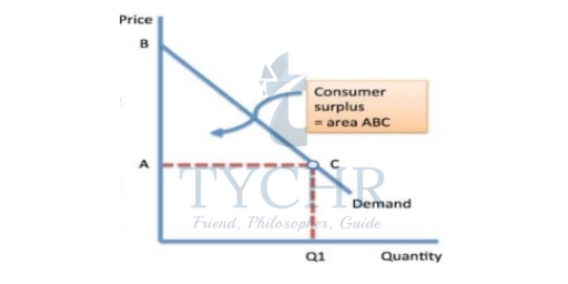
A Consumer surplus is indicated by the area under the demand curve and above the market price.
PRODUCER SURPLUS
Producer surplus is a measure of producer welfare
Producer surplus is the difference between what producers are willing and able to supply a good for and the price they actually receive.
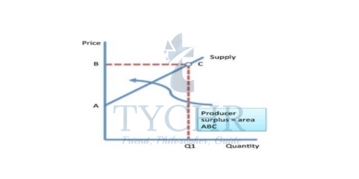
Producer surplus shown by area above the supply curve and below the market price.
Higher prices provide an incentive to supply more to the market (profit motive)
COMPETITIVE MARKET EQUILIBRIUM (SOCIAL SURPLUS)
The definition of it is the sum of consumer surplus and producer surplus at its highest point.
MARKET EQUILIBRIUM & ALLOCATIVE EFFICIENCY
In competitive market equilibrium, as shown in the above figure, production of goods occurs where MB=MC, also the point of Social Surplus.
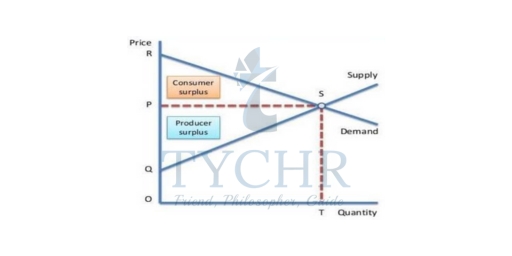
This means that markets are achieving Allocative as well as productive efficiency, producing the quantity of goods wanted by the society at the lowest possible cost. Optimum utilization of resources is being done.
A word of Caution!
In the above topic, we have discussed that the market achieves equilibrium without government interference. But in reality it has failed, mainly due to 2 reasons:
The government needs to interfere, because efficiency can be realized only under stringent conditions.
Whom to produce works significantly when the government interferes in relation to output and income distribution.