By the end of this chapter you should be familiar with:
- Antiderivative
- Indefinite integral
- Upper limit and lower limit
- Definite integral
- Numerical integration
- Reverse rule
- Area under the curve
- Volumes of revolution
- Exact solutions of differential equations
- Slope fields
- Euler’s method
INDEFINITE INTEGRALS
Given a function, f(x), an anti-derivative of f(x) is any function F(x) such that F′(x) = f(x)
If F(x) is any anti-derivative of f(x) then the most general anti-derivative of f(x) is called an indefinite integral and denoted by ∫ f(x)dx= F(x) + c
In this definition the ∫ is called the integral symbol, f(x) is called the integrand, x is called the integration variable and the c is called the constant of integration.
dx means that we are going to integrate our function w.r.t x. Constant c is a must.
Example: Evaluate the following indefinite integral ∫𝑥4 + 3x − 9 dx
Solution: The indefinite integral is,
∫𝑥4 + 3x − 9 dx = (1/5)x5 +(3/2)x2 – 9x + c
Here is a table showing some integrals of common functions as anti-derivatives:

PROPERTIES
Let F and G be antiderivatives of f and g, respectively, and let k be any real number.
Sums and Differences
∫f(x)±g(x)= F(x) ± G(x) + C
Constant Multiples
∫ kf(x) dx= kF(x) + C
SUBSTITUTION RULE
Integration by Substitution is a method to find an integral, but only when it can be set up in a special way. Given by: ∫ f(g(x)) g′(x) dx = ∫ f(u) du
where u=g(x)
Integration by parts also known as the chain rule is given by∫ 𝑢 𝑑𝑣 = uv – ∫ 𝑣 𝑑𝑢
Example: Evaluate the following integrals:
- ∫ (1 − (1/w)) cos(w − lnw)dw
- ∫ 𝑥 𝑑𝑥/√1−4𝑥2
Solution:
- In this case it looks like we have a cosine with an inside function and so let’s use that as the substitution.
u = w − lnw
du = (1 – 1/w) dw
∫ (1 − (1/w)) cos(w − lnw) dw = ∫ cos 𝑢 𝑑𝑢
= sin u + c
= sin(w − lnw) + c - In this example don’t forget to bring the root up to the numerator and change it into fractional exponent form. Upon doing this we can see that the substitution is,
u = 1 − 4x2
du = −8x dx
x dx = −18du
∫ 𝑥 𝑑𝑥/√(1−4𝑥2)= ∫ 𝑥(1 − 4𝑥2)−1/2 𝑑𝑥
= (−1/8) ∫𝑢−1/2𝑑𝑢
=(-1/4) u1/2 + c
= (-1/4)√(1 − 4𝑥2) + c
SOME APPLICATIONS TO ECONOMICS
- Cost function: C(x) = total cost of producing x units of a product during some time period.
- Revenue function: R(x) = total revenue from selling x units of the product during the time period.
- Profit function: P(x) = total profit obtained by selling x units of the product during the time period.
P(x) = R(x) – C(x)
The total cost C(x) of producing x units is made up of two parts: overhead or fixed costs, a, and variable costs or manufacturing cost, M(x).
C(x) = a + M(x)
If a firm can sell all the items it produces p units of money each, then
R(x) = px
Also all economists call, P’(x), R’(x), C’(x) the marginal profit, marginal revenue and marginal cost.
R(x) – C(x) ≥ 0. An investment is valuable until R’(x) = C’(x) since beyond this point, the marginal cost will be more than the revenue.
Example: The marginal revenue of a company is given by MR = 100 + 20Q + 3Q2, where Q is the amount of units sold for a period. Find the total revenue function if at Q = 2 it is equal to 260.
Solution: We find the total revenue function TR by integrating the marginal revenue function MR:
TR(Q) = ∫ MR(Q) dQ
= ∫ 100 + 20Q + 3𝑄2 𝑑𝑄
= 100Q + 10Q2 + Q3 + c
The constant of integration c can be determined using the initial condition
TR(Q=2) = 260.
Hence, 200 + 40 + 8 + C =260
C=12
So, the total revenue function is given by
TR(Q) = Q3 + 10Q2 + 100Q + 12
AREA AND THE DEFINITE INTEGRAL
The area problem will give us one of the interpretations of a definite integral and it will lead us to the definition of the definite integral.
To start off we are going to assume that we’ve got a function f(x) that is positive on some interval [a, b]. What we want to do is determine the area of the region between the function and the x-axis.
Lets take an example to understand:
Determine the area between f(x) = x2 + 1 on [0,2]. In other words, we want to determine the area of the shaded region below
Δx = (b − a)/n
Then in each interval we can form a rectangle whose height is given by the function value at a specific point in the interval. We can then find the area of each of these rectangles, add them up and this will be an estimate of the area.
It’s probably easier to see this with a sketch of the situation. So, let’s divide up the interval into 4 subintervals and use the function value at the right endpoint of each interval to define the height of the rectangle. This gives,

A = (1/2) f(1/2) + (1/2) f(1) + (1/2) f(3/2) + (1/2) f(2) A = 5.75
Of course, taking the rectangle heights to be the function value at the right endpoint is not our only option. We could have taken the rectangle heights to be the function value at the left endpoint. Using the left endpoints as the heights of the rectangles will give the following graph and estimated area.
A = (1/2) f(1/2) + (1/2) f(1) + (1/2) f(3/2) + (1/2) f(2) A = 3.75
In this case we can see that the estimation will be an underestimation since each rectangle misses some of the area each time.
There is one more common point for getting the heights of the rectangles that is often more accurate. Instead of using the right or left endpoints of each sub interval we could take the midpoint of each subinterval as the height of each rectangle. Here is the graph for this case.
So, it looks like each rectangle will over and under estimate the area. This means that the approximation this time should be much better than the previous two choices of points. Here is the estimation for this case.
A = (1/2) f(1/2) + (1/2) f(1) + (1/2) f(3/2) + (1/2) f(2) A = 4.625
The easiest way to get a better approximation is to take more rectangles (i.e. increase n). Let’s double the number of rectangles that we used and see what happens. Here are the graphs showing the eight rectangles and the estimations for each of the three choices for rectangle heights that we used above.


A = 4.65
So, increasing the number of rectangles did improve the accuracy of the estimation.
DEFINITE INTEGRAL
Given a function f(x) that is continuous on the interval [a,b] we divide the interval into n sub-intervals of equal width, Δx, and from each interval choose a point, xi. Then the definite integral of f(x) from a to b is:

The number “a” that is at the bottom of the integral sign is called the lower limit of the integral and the number “b” at the top of the integral sign is called the upper limit of the integral. Also, despite the fact that aa and bb were given as an interval the lower limit does not necessarily need to be smaller than the upper limit. Collectively we’ll often call a and b the interval of integration.
PROPERTIES
 We can interchange the limits on any definite integral, all that we need to do is tack a minus sign onto the integral when we do.
 If the upper and lower limits are the same then there is no work to do, the integral is zero.
 where c is any number. So, as with limits, derivatives, and indefinite integrals we can factor out a constant.
 We can break up definite integrals across a sum or difference.
 where c is any number. This property is more important than we might realize at first. One of the main uses of this property is to tell us how we can integrate a function over the adjacent intervals, [a, c] and [c, b]. Note however that c doesn’t need to be between a and b.
 The point of this property is to notice that as long as the function and limits are the same the variable of integration that we use in the definite integral won’t affect the answer.
Suppose f(x) is a continuous function on [a, b] and also suppose that F(x) is any anti-derivative for f(x). Then,

Example: Evaluate the following
Solution:
- ∫1−3 6𝑥2 − 5𝑥 + 2 𝑑𝑥 = (2x3 – (5/2)x2 + 2x)|1−3
= (2 – (5/2) + 2) – ( -54 – (45/2) – 6)
= 84 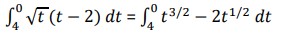
USING SUBSTITUTION WITH DEFINITE INTEGRAL
We are going to be using the same steps as we used for indefinite integral but here there will be a change in the limits according to the substitution taken. Lets take an example to understand.
Example: Evaluate ∫0(1+ 𝜋) 𝑒𝑥cos(1 − 𝑒𝑥)𝑑𝑥
Solution: u = 1 – ex du = -ex dx
when x = 0, u = 1 – 1 = 0
when x = ln(1 + π), u = 1 – eln(1 + π) = 1 – (1 + π) = -π
MIDPOINT RULE
We will divide the interval [a,b] into n sub-intervals of equal width,
Δx = (b−a)/n
We will denote each of the intervals as follows,
[x0, x1], [x1, x2], …, [xn−1, xn] where x0 = a and xn = b
Then for each interval let xi be the midpoint of the interval. We then sketch in rectangles for each subinterval with a height of f(xi). Here is a graph showing the set up using n=6.
We can easily find the area for each of these rectangles and so for a general n we get that,
∫𝑏𝑎 𝑓(𝑥) 𝑑𝑥 = Δx[ f(x1) + f(x2) + ⋯ + f(xn)]
TRAPEZOIDAL RULE
For this rule we will do the same set up as for the Midpoint Rule. We will break up the interval [a,b] into n sub-intervals of width,
Δx = (b − a)/n
Then on each subinterval we will approximate the function with a straight line that is equal to the function values at either endpoint of the interval. Here is a sketch of this case for n=6.
The area of the trapezoid in the interval [xi-1, xi] is given by,
Ai = (Δx/2) (f(xi-1) + f(xi))
Upon doing a little simplification we arrive at the general Trapezoid Rule:
∫𝑏𝑎 𝑓(𝑥) 𝑑𝑥 = (∆𝑥/2)[ f(x0) + 2f(x1) + 2f(x2) ⋯ + 2f(xn-1) + f(xn)]
Example: Using trapezoidal rule with n=4 evaluate ![]()
Solution: Δx = (2 – 0)/4 = 1/2
And so the sub-intervals will be [0, 0.5], [0.5, 1], [1, 1.5], [1.5, 2]
Using the trapezoidal rule,
CONTINUOUS MONEY FLOW
TOTAL MONEY FLOW: If f(t) is the rate of money flow, then the total money flow over the time interval t = 0 to t = T is given by
Total = ∫𝑇0 𝑓(𝑡) 𝑑𝑡
It is vital to note the difference between the variable t, and the fixed amount of time, T (a constant).
PRESENT VALUE OF MONEY FLOW: If f(t) is the rate of continuous money flow at an interest rate r, compounded continuously for T years, then the present value is
P = ∫𝑇0𝑓(𝑡) 𝑒−𝑟𝑡 𝑑𝑡
ACCUMULATED AMOUNT OF MONEY FLOW AT TIME T: If f(t) is the rate of money flow at an interest rate r, at time t, the accumulated amount of money flow at time T is
FV = erT∫𝑇0𝑓(𝑡) 𝑒−𝑟𝑡 𝑑𝑡
Example: At what constant, continuous rate must money be deposited into an account if the account contains $20,000 in 5 years? The account earns 6% interest compounded continuously.
Solution: Given FV = $20, 000, M = 5, r = 0.06. S is assumed to be constant then we have,
20000 = S∫50 𝑒−0.06𝑡 𝑑𝑡
S = 20000/4.319 = $4,630 per year.
AREAS
AREA BETWEEN A CURVE AND X-AXIS
When calculating the area between a curve and the x-axis, you should carry out separate calculations for the parts of the curve above the axis, and the parts of the curve below the axis. The integral for a part of the curve below the axis gives minus the area for that part. You may find it helpful to draw a sketch of the curve for the required range of x-values, in order to see how many separate calculations will be needed. Lets say the curve is some y. The area is given by:
A = ∫ba y𝑑x
Example: Find the area between the curve y = x(x − 3) and the ordinates x = 0 and x = 5.
Solution: If we set y = 0 we see that x(x − 3) = 0, and so x = 0 or x = 3. Thus, the curve cuts the x-axis at x = 0 and at x = 3. The x 2 term is positive, and so we know that the curve forms a U-shape as shown below.
From the graph, we can see that we need to calculate the area A between the curve, the x-axis and the ordinates x = 0 and x = 3 first, and that we should expect this integral to give a negative answer because the area is wholly below the x-axis:
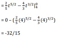
A = ∫30𝑦 𝑑𝑥= ∫ 𝑥2 − 3𝑥 𝑑𝑥
= 𝑥3/3 − 3𝑥2/2|03
= 9 – (27/2) = -9/2
Next, we need to calculate the area B between the curve, the x-axis, and the ordinates x = 3 and x = 5:
A = ∫53𝑦 𝑑𝑥= ∫53𝑥2 − 3𝑥 𝑑𝑥
= 𝑥3/3 − 3𝑥2/2|53
= (125/3) – (125/2) – ((27/3) – (27/2))
= 26/3
Total Area = 26/3 – 9/2
= 25/6 units of area.
AREA BETWEEN TWO CURVES
A similar technique to the one we have just used can also be employed to find the areas sandwiched between curves. The area is given by:
A = ∫ba|𝑓(𝑥) − 𝑔(𝑥)| 𝑑𝑥
Example: Calculate the area of the segment cut from the curve y = x(3 − x) by the line y = x.
Solution: Sketching both curves on the same axes, we can see by setting y = 0 that the curve y = x(3−x) cuts the x-axis at x = 0 and x = 3. Furthermore, the coefficient of x2 is negative and so we have an inverted U-shape curve. The line y = x goes through the origin and meets the curve y = x(3 − x) at the point P. It is this point that we need to find first of all.
At P the y co-ordinates of both curves are equal. Hence:
x(3 − x) = x 3x – x2 = x 2x – x2 = 0 x(2 − x) = 0
so that either x = 0, the origin, or else x = 2, the x co-ordinate of the point P. We now need to find the shaded area in the diagram. To do this we need the area under the upper curve, the graph of y = x(3 − x), between the x-axis and the ordinates x = 0 and x = 2. Then we need to subtract from this the area under the lower curve, the line y = x, and between the x-axis and the ordinates x = 0 and x = 2. The area under the curve is:
A = ∫20 𝑦 𝑑𝑥 = ∫20 −𝑥 2 + 3𝑥 𝑑𝑥 = – 𝑥3/3 + 3𝑥2/2 |0 2
= 6 – (8/3) = 10/3
and the area under the straight line is:
A =∫20 𝑦 𝑑𝑥 = ∫20 𝑥 𝑑𝑥
= 𝑥2/2|02 = 2 – 0 = 2
Thus, the area of the shaded region = (10/3) – 2
= 4/3 units of area.
SOLIDS OF REVOLUTION
METHOD OF RINGS
To get a solid of revolution we start out with a function, y=f(x), on an interval [a, b].
We then rotate this curve about a given axis to get the surface of the solid of revolution. For purposes of this discussion let’s rotate the curve about the x-axis, although it could be any vertical or horizontal axis. Doing this for the curve above gives the following three-dimensional region.
The volume of this solid is given by:
V = ∫𝑏𝑎 𝐴(𝑥) 𝑑𝑥 or V = ∫𝑑𝑐 𝐴(𝑦) 𝑑𝑦
where, A(x) and A(y) is the cross-sectional area of the solid which is
A = π((r2)2 – (r1)2) where, r1 = outer radius and r2 = inner radius.
Example: Determine the volume of the solid obtained by rotating the portion of the region bounded by y = and y = x/4 that lies in the first quadrant about the y-axis.
Solution: First, let’s get a graph of the bounding region and a graph of the object. Remember that we only want the portion of the bounding region that lies in the first quadrant. There is a portion of the bounding region that is in the third quadrant as well, but we don’t want that for this problem.

Next, we will get our cross section by cutting the object perpendicular to the axis of rotation. The cross section will be a ring (remember we are only looking at the walls) for this example and it will be horizontal at some y. This means that the inner and outer radius for the ring will be x values and so we will need to rewrite our functions into the form x = f(y).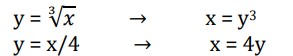 Here are a couple of sketches of the boundaries of the walls of this object as well as a typical ring. The sketch on the left includes the back portion of the object to give a little context to the figure on the right.

A(y) = π((4y)2 – (y3)2)
= π(16y2 – y6)
Working from the bottom of the solid to the top we can see that the first cross-section will occur at y=0 and the last cross-section will occur at y=2. These will be the limits of integration. The volume is then,
METHOD OF CYLINDERS
The volume formula stays the same as the method of rings but the area differs.
A = 2πrh where r = radius and h = height
Example: Determine the volume of the solid obtained by rotating the region bounded by x = (y−2)2 and y = x about the line y = -1.
Solution: We should first get the intersection points there.
y = (y − 2)2
y = y2 − 4y + 4
0 = (y − 4)(y − 1)
So, the two curves will intersect at y = 1 and y = 4. Here is a sketch of the bounded region and the solid.

Here are our sketches of a typical cylinder. The sketch on the left is here to provide some context for the sketch on the right.

A(y) = 2πrh = 2π(y + 1)(y − (y − 2)2) = 2π(−y3 + 4y2 + y − 4)
The first cylinder will cut into the solid at y = 1 and the final cylinder will cut in at y = 4. The volume is then,
As already seen in previous chapters, we know that
displacement (s) → [ds/dt] → velocity (v) → [dv/dt] → acceleration (a)
displacement (s) ← [ ∫v dt] ← velocity (v) ← [ ∫a dt] ← acceleration (a)
Example: The velocity of a particle is modelled by v(t) = 3t2 + 5t, where t is measured in seconds. Find the displacement of the particle after 5 seconds.
Solution: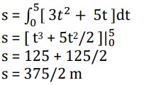
Area under a velocity-time graph can be calculated using definite integrals but with the form:
∫𝑏𝑎 𝑎(𝑡) 𝑑𝑥 = v(b) – v(a) or ∫𝑏𝑎 𝑎(𝑡) 𝑑𝑥 = s(b) – b(a)
DIFFERENTIAL EQUATIONS
A differential equation is an equation that contains a derivative.
A separable differential equation is any differential equation that we can write in the following form:
N(y) (dy/dx) = M(x)
To solve this differential equation we first integrate both sides with respect to x to get,

Example: Solve the following differential equation y′ = e-y (2x−4) with y(5)=0
Solution: This differential equation is easy enough to separate, so let’s do that and then integrate both sides.
ey dy = (2x – 4) dx
∫ 𝑒𝑦 𝑑𝑦 = ∫ 2𝑥 − 4 𝑑𝑥
ey = x2 – 4x + c
Applying the initial condition gives
1 = 25 – 20 + c c = −4
This then gives an implicit solution of
ey = x2 – 4x – 4
We can easily find the explicit solution to this differential equation by simply taking the natural log of both sides.
y(x) = ln(x2 – 4x – 4)
SLOPE FIELDS AND DIFFERENTIAL EQUATIONS
- Slope fields are visual representations of differential equations of the form dy/dx = f(x, y).
- At each sample point of a slope field, there is a segment having slope equal to the value of dy/dx.
- Any curve that follows the flow suggested by the directions of the segments is a solution to the differential equation.
Example:
Consider dy/dt = f(y) where f(y) is given by the graph shown below. Sketch the slope fields of this differential equation
Solution: Since we do not know the function f(y), we will only be able to sketch the slope fields. This will give us an idea about the behaviour of the solutions. Therefore, we should be looking for the critical solutions (given by the roots of f(y)=0), and the sign of f(y) which will give the variation of the solutions. Note that we should be careful not to mix between the graph of f(y) and the graphs of the solutions y(t).
So, according to the graph of f(y), the critical solutions are y = -1, y = 0, and y = 1. Using the sign of f(y), we conclude that:
- The solutions located in the region y < -1 are decreasing,
- The solutions located in the region -1 < y <0 are increasing,
- The solutions located in the region 0 < y < 1 are decreasing,
- The solutions located in the region 1 < y are increasing.
The sketch of the slope fields is given below.
EULER’S METHOD
Consider the differential equation dy/dt = f(t, y) with y(t0) = y0
where f(t, y) is a known function and the values in the initial condition are also known numbers. We know that if f and fy are continuous functions then there is a unique solution to the differential equation in some interval surrounding t = t0. So, let’s assume that everything is continuous so that we know that a solution will in fact exist.
We want to approximate the solution near t = t0 and can write the tangent line as:
y = y0 + f(t0, y0)(t−t0)

If we have tn and the approximation to the solution at this point, yn, and we want to find the approximation at tn+1 all we need to do is use the following.
yn+1 = yn + f(tn, yn)⋅(tn+1 – tn)
After approximations and substitutions Euler’s formula is given by:
yn = yn-1 + h f(tn-1, yn-1).
Example: Use Euler’s Method for y’ = xy with y(1) = 1 and a step size of h=0.1 to find approximate value of y(2).
Solution:
Using yn = yn-1 + h f(xn-1, yn-1)
h = 0.1, f(x,y) = xy
Hence,
yn = yn-1 + 0.1(xn-1 × yn-1)
yn = yn-1(1 + 0.1xn-1)
y(2) = y(1) ( 1 + 0.1 x(1))
y(2) = 3.86
