IB Math AI HL Paper 2 Question Bank
IB Math AI HL Paper 2 Question Bank is a great resource for students who are preparing for their IB Math AI HL Paper 2 exam. The question bank offers a wide range of questions, from easy to difficult, that cover all the topics in the IB Math AI HL syllabus. This is an essential tool for students who want to score well in their paper 2 exam. Take a look around and see what we have to offer – we think you’ll be impressed!
1.) The family of curves y = f(x) = (ax3 + bx2 + cx + d)n, where a, b, c, d, and n are constants, is given.
a) For n = 2, determine the inflection point of the function y = f(x).
For n = 2, the function becomes y = (ax3 + bx2 + cx + d)2. To find the inflection point, we need to find the second derivative of the function, which is:
f”(x) = 6a2x + 2b
Now we need to find the x values where the second derivative is equal to zero.
6a2x + 2b = 0
x = -b/(3a2)
b) Next, Consider the curve, y2 = 2x3 + x
i) Find the derivative of y2 = 2x3 + x
y2 = 2x3 + x
y = √(2x3 + x)
Next, we can take the derivative of this expression using the chain rule. The chain rule states that if we have a function u(x) = f(g(x)), then the derivative of u(x) with respect to x is given by:
du/dx = df/dg * dg/dx
In this case, we have u(x) = sqrt(2x3 + x) and we have to find the derivative of this function with respect to x
du/dx = (1/2)(2x3 + x)(-1/2)(6x2 + 1) = (3x(2x2 + 1))/(2√(2x3 + x))
So the derivative of y = sqrt(2x3 + x) with respect to x is (3x(2x2 + 1))/(2√(2x3 + x))
ii) Hence, find the local minima or maxima of y2 = 2x3 + x
To find the local maxima or minima of y2 = 2x3 + x, we need to find the critical points of the function
y = √(2x3 + x).
A critical point of a function is a point where the derivative of the function is equal to zero or does not exist.
First, we need to find the derivative of y = √(2x3 + x) with respect to x:
y’ = (3x(2x2 + 1))/(2√(2x3 + x))
Next, we need to set y’ equal to zero and solve for x:
(3x(2x2 + 1))/(2√(2x3 + x)) = 0
3x(2x2 + 1) = 0
x = 0
Now, we need to check if x = 0 is a local maximum or minimum. To do this, we need to find the second derivative of y = √(2x3 + x) with respect to x:
y” = (6x(2x2 + 1) – 3(2x2 + 1)(2x))/ (2√(2x3 + x))2
We need to evaluate y” at x = 0, we get
y”(0) = -3/2, which is negative and that means that x = 0 is a local minimum.
So the local minima of y2 = 2x3 + x is (0, 0)
2.) An amount of $ 10 000 is invested at an annual interest rate of 12%.
a) Find the value of the investment after 5 years
i) if the interest rate is compounded yearly;
FV=10000(1+12/100)n
n= 5, 17623.42
ii) if the interest rate is compounded half-yearly;
n= 10, 17908.48
iii) if the interest rate is compounded quarterly;
n=20, 18061.11
iv) if the interest rate is compounded monthly.
n= 5*12, 18166.97
b) The value of the investment will exceed $ 20 000 after n full years. Calculate the minimum value of n
i) if the interest rate is compounded yearly;
20000= 10000(1+12/100)n
Solve by GDC
n=6.11, hence n=7
ii) if the interest rate is compounded monthly.
20000= 10000(1+12/100)12n
Solve by GDC
n=5.81, hence n=6
3.) In the triangle PQR, PR = 5 cm, QR = 4 cm and PQ = 6 cm. Calculate
a) The size of PQR
52 = 42 + 62 – 2(4)(6)(cosQ)
PQR = 55.8°
b)The area of the triangle PQR
½ (4)(6)(sin55.8)= 9.92cm2
4.) O is the centre of the circle which has a radius of 5.4 cm.
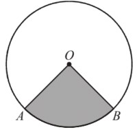
Area of the shaded sector OAB is 21.6 cm2. Find the length of the minor arc AB
½(5.4)2𝜃 = 21.6
𝜃 = 1.481 radians
AB = r𝜃 = 5.4*1.481 = 8cm
5.) Consider the geometric sequence 10, 5, 2.5, 1.25, …
a) Write down the first term u1 and the common ratio r.
u1= 10, r= 0.5
b) Find the 10th term of the sequence.
0.0195
c) Find the sum of the first 10 terms.
19.98
d) Express the general term un in terms of n.
10*0.5(n-1)
(e) Hence find the value of n given that un.03125
n= 6

6.) An amount of $ 10 000 is invested at an annual interest rate of 12%.
a) Find the value of the investment after 5 years
i) if the interest rate is compounded yearly;
FV=10000(1+12/100)n
n= 5, 17623.42
ii) if the interest rate is compounded half-yearly;
n= 10, 17908.48
iii) if the interest rate is compounded quarterly;
n=20, 18061.11
iv) if the interest rate is compounded monthly.
n= 5*12, 18166.97
b) The value of the investment will exceed $ 20 000 after n full years. Calculate the minimum value of n
i) if the interest rate is compounded yearly;
20000= 10000(1+12/100)n
n=6.11, hence n=7
ii) if the interest rate is compounded monthly.
20000= 10000(1+12/100)12n
n=5.81, hence n=6
7.) Let f(x) = ex – x2 and g(x) = x3 – 3x2 + 2x + 1
a) Find the derivative of f(x) using the chain rule and the product rule.
f'(x) = ex – 2x
b) Find the derivative of g(x) using the power rule
g'(x) = 3x2 – 6x + 2
c) Find the point(s) of the intersection of the graphs of y = f(x) and y = g(x) and state whether they are minima or maxima.
The point(s) of intersection can be found by solving the equation f(x) = g(x), which gives x = 0.5 and x = -0.5. Since the second derivative of f(x) at those points is positive, it follows that the points of intersection are minima.
d) Find the second derivative of f(x) and express it in terms of x.
f”(x) = ex – 2
e)Using the information from parts 1-4, determine the concavity of the graph of y = f(x) and state the point(s) of inflection.
The second derivative of f(x) is positive for x < -0.5 and x > 0.5, it follows that f(x) is concave up on those intervals, and therefore the points of inflection are x = -0.5 and x = 0.5.
8.) The weight X of a particular animal is normally distributed with μ= 200kg and σ= 15kg. An animal of this population is overweight if it has a weight greater than 230 kg
a) Find the probability that an animal is overweight.
P (X>230) = 0.02275
b) We select 2 animals from this population. Find the probabilities that
i) both animals are overweight
(0.02275)2 = 0.000518
ii) only one animal is overweight.
0.02275)* (1-0.02275)* 2 = 0.0445
c) We select 7 animals from this population. Find the probability that exactly two of them are overweight.
Y follows B(n,p) with n = 7, p =0.02275
P(Y=2) = 0.00969
9.) A factory produces mobile components, where the probability of a component being defective is 0.05. The factory produces 1000 components per day.
a) Use the binomial distribution to find the probability that exactly 50 components are defective in a day.
P(X = 50) = (1000 C 50) * (0.05)50 * (1-0.05)950
p(X = 50) = 0.09
b) Use the binomial distribution to find the probability that less than 50 components are defective in a day.
P(X < 50) = P(X = 0) + P(X = 1) + P(X = 2) + … + P(X = 49)
c) Use the Poisson distribution to find the probability that exactly 50 components are defective in a day.
P(X = 50) = (e-5 * 550) / 50!
d) Compare the results obtained in parts 1 and 3 and explain the conditions under which
the Poisson distribution can be used to approximate the binomial distribution.
Poisson distribution can be used as an approximation of the binomial distribution when the number of trials is large and the probability of success is small
e) Find the expected value and standard deviation of the number of defective components produced in a day.
E(X) = n * p = 1000 * 0.05 = 50 and σ = √(np(1-p)) = √(1000 * 0.05 * 0.95) = 4.72
10.) A factory produces mobile components, where the probability of a component being defective is 0.05. The factory produces 1000 components per day.
a) Use the binomial distribution to find the probability that exactly 50 components are defective in a day.
P(X = 50) = (1000 C 50) * (0.05)50 * (1-0.05)950
p(X = 50) = 0.09
b) Use the binomial distribution to find the probability that less than 50 components are defective in a day.
P(X < 50) = P(X = 0) + P(X = 1) + P(X = 2) + … + P(X = 49)
c) Use the Poisson distribution to find the probability that exactly 50 components are defective in a day.
P(X = 50) = (e-5 * 550) / 50!
d) Compare the results obtained in parts 1 and 3 and explain the conditions under which
The Poisson distribution can be used to approximate the binomial distribution.
Poisson distribution can be used as an approximation of the binomial distribution when the number of trials is large and the probability of success is small
e) Find the expected value and standard deviation of the number of defective components produced in a day.
E(X) = n * p = 1000 * 0.05 = 50 and σ = √(np(1-p)) = √(1000 * 0.05 * 0.95) = 4.72
11.) Tony wants to be able to complete 57 pullups in one go without a break. He sets out a training regime whereby he completes 5 pullups on the first day, then adds 5 pullups each day thereafter.
a) Write down the number of pushups Charles completes on the 6th training day.
On the 6th training day, Tony completes 5 + 5(6-1) = 5 + 5(5) = 5 + 25 = 30 pullups.
b) Find an expression for the number of pushups Charles completes on the nth training day.
The number of pullups Tony completes on the nth training day can be expressed as: 5 + 5(n-1).
c) On the kth training day, Charles completes 57 pull ups for the first time. Find the value of k.
Since Tony completes 57 pullups for the first time on the kth training day, we can set up the equation: 5 + 5(k-1) = 57. Solving for k, we get: k = 12.
d) Calculate the total number of pushups Charles completes on the first 8 training days.
To calculate the total number of pullups Tony completes on the first 8 training days, we can use the formula for the sum of an arithmetic series: Sum = n/2 * (2a + (n-1)d), where n is the number of terms, a is the first term, and d is the common difference. Plugging in the values, we get: Sum = 8/2 * (2*5 + (8-1)*5) = 4 * (10 + 35) = 180 pullups.
Charles is also working on improving his long distance running in preparation for a marathon event in 7 weeks time. He runs a total of 8,000 meters in the first week and plans to increase this by 6% each week up until the event.
e) Find the distance Charles swims in the 4th week of training.
Tony plans to increase his running distance by 6% each week. So, the distance he runs in the 4th week can be calculated as: 8,000 * 1.06^3 = 8,000 * 1.191016 = 9,528.13 meters (rounded to the nearest meter).
f) Calculate the total distance Charles runs until the event.
To calculate the total distance Tony runs until the event in 7 weeks, we can again use the formula for the sum of an arithmetic series. Plugging in the values, we get: Sum = 7/2 * (2*8,000 + (7-1)*6% * 8,000) = 3.5 * (16,000 + 3,360) = 67,760 meters.
12.) Consider a 3×3 matrix A that represents a linear transformation. The matrix A can be subdivided into three 2×2 matrices as shown below:
A = [B C D]
[E F G]
[H I J]
The matrix A has eigenvalues λ₁ = 3, λ₂ = 1, and λ₃ = -2, with corresponding eigenvectors v₁ = [1, 0, 1], v₂ = [0, 1, 1], and v₃ = [1, 1, 0], respectively.
a) Find the eigenvalues and eigenvectors of each 2×2 matrix B, C, D, E, F, G, H, I, and J.
To find the eigenvalues and eigenvectors of each 2×2 matrix, we can extract the corresponding submatrices and follow the process mentioned earlier.
For matrix B:
B = [B₁ B2]
[B3 B4]
Substituting the values, we have:
B = [B₁ B2]
[B3 B4]
To find the eigenvalues, we solve the characteristic equation:
|B – λI| = 0
Substituting the values, we have:
|B – λI| = |B₁ – λ B2|
[B3 B4 – λ| = 0
Expanding the determinant, we get:
(B₁ – λ)(B₄4 – λ) – B2B3 = 0
Simplifying the equation, we have:
λ² – (B₁ + B4)λ + (B₁B4 – B2B3) = 0
The solutions to this equation are the eigenvalues of matrix B. Once we find the eigenvalues, we can find the corresponding eigenvectors by solving the system of equations:
(B – λI)v = 0
Using the same process, we can find the eigenvalues and eigenvectors for matrices C, D, E, F, G, H, I, and J.
b) Suppose that matrix A represents a transformation in 3D space. The matrix A scales vectors by a factor of 2 along the eigenvector v₁ reflects vectors across the plane defined by the eigenvector v2, and shears vectors along the eigenvector v₃.
(i) Explain how the eigenvalues and eigenvectors of A relate to the scaling, reflection, and shearing properties described above.
The eigenvalue λ₁ = 3 indicates that the transformation scales vectors by a factor of 3 along the eigenvector v₁ = [1, 0, 1]. This means that vectors in the direction of v₁ will be elongated or stretched by a factor of 3.
The eigenvalue λ2 = 1 represents the reflection property of matrix A. It reflects vectors across the plane defined by the eigenvector v2 = [0, 1, 1]. Any vector lying in the plane spanned by v2 will remain the same under the transformation, while vectors perpendicular to v2 will be flipped or reflected.
The eigenvalue λ3 = -2 signifies the shearing property. The transformation shears vectors along the eigenvector v3 = [1, 1, 0], distorting their shapes without changing their lengths.
(ii) To determine the transformation matrix representing the scaling, reflection, and shearing operations, we combine the effects of each eigenvector’s transformation.
The transformation matrix can be constructed as follows:
A = [3v1 v2 v3]
Substituting the given eigenvector values, we have:
A = [3(1, 0, 1) (0, 1, 1) (1, 1, 0)]
Simplifying, we get:
A = [3 0 3]
[0 1 1]
[3 3 0]
This transformation matrix A will scale vectors by a factor of 3 along the direction of v₁ = [1, 0, 1], reflect vectors across the plane defined by v₂ = [0, 1, 1], and shear vectors along the direction of v₃ = [1, 1, 0].
13.) Consider the function f(x) = x3 – 3x2 – 9x + 1.
a) Find the stationary points of f(x). Determine the nature of each stationary point, giving reasons for your answer.
To find the stationary points, we need to find where the derivative of the function is equal to zero:
f'(x) = 3x2 – 6x – 9 = 3(x – 3)(x + 1)
Setting f'(x) = 0 gives us the stationary points at x = -1 and x = 3. To determine the nature of each stationary point, we need to examine the sign of the second derivative:
f”(x) = 6x – 6
At x = -1, f”(-1) = -12, so the stationary point at x = -1 is a local maximum.
At x = 3, f”(3) = 12, so the stationary point at x = 3 is a local minimum.
Therefore, the stationary points of f(x) are (-1, 14) and (3, -19), where the y-values are found by plugging in the x-values into the original function.
b) Sketch the graph of y = f(x), showing clearly the coordinates of all stationary points and any points of inflection.
To sketch the graph, we can start by plotting the stationary points (-1, 14) and (3, -19). We can also find the point of inflection by setting the second derivative equal to zero:
f”(x) = 6x – 6 = 0
x = 1
So the point of inflection is (1, -10). We can now use this information to sketch the graph:
The points of inflection are not labeled, but occur at approximately x = -1.28 and x = 2.62.
c) Determine the intervals on which f(x) is increasing and decreasing.
To find the intervals on which f(x) is increasing and decreasing, we can examine the sign of the first derivative:
f'(x) = 3x2 – 6x – 9 = 3(x – 3)(x + 1)
On the interval (-∞, -1), f'(x) is negative, so f(x) is decreasing.
On the interval (-1, 3), f'(x) is positive, so f(x) is increasing.
On the interval (3, ∞), f'(x) is positive, so f(x) is increasing.
Therefore, f(x) is decreasing on (-∞, -1) and increasing on (-1, 3) and (3, ∞).
14.) A particle P moves in space such that its position vector r(t) at time t seconds is given by:
r(t) = (3t + 2)i + (t2 – 1)j + (4t – 3)
a) Find the velocity vector v(t) of P.
The velocity vector is the derivative of the position vector:
v(t) = r'(t) = 3i + 2tj + 4k
b) Find the speed of P at time t = 2 seconds.
The speed of the particle at time t = 2 seconds is the magnitude of its velocity vector at that time:
|v(2)| = √(32 + 2(2)2 + 42) = √29
c) Find the equation of the line of motion of P.
To find the equation of the line of motion, we need a point on the line and a direction vector. We can take r(0) = 2i – j – 3k as a point on the line, and v(t) as the direction vector:
r(t) = (3t + 2)i + (t2 – 1)j + (4t – 3)k
r(0) = 2i – j – 3k
v(t) = 3i + 2tj + 4k
So the equation of the line is:
r = (2 + 3s)i + (s2 – 1)j + (-3 + 4s)k
d) At time t = 2 seconds, P is on the line L: r = (4 + s)i + (3 – 2s)j + (s – 2)k. Determine the value of s and the shortest distance from P to L.
We are given that P is on the line L: r = (4 + s)i + (3 – 2s)j + (s – 2)k when t = 2 seconds, so we can substitute t = 2 into the equation for r(t) to find the position vector of P at that time:
r(2) = (3(2) + 2)i + ((2)2 – 1)j + (4(2) – 3)k
= 8i + 3j + 5k
We want to find the value of s that makes r(2) equal to a point on the line L. Equating the corresponding components, we have:
8 = 4 + s
3 = 3 – 2s
5 = s – 2
The second equation tells us that s = 0. However, this does not satisfy the other two equations, so there is no point on L that is equal to r(2).
Therefore, the shortest distance from P to L is the perpendicular distance between the line and the point r(2). This distance can be found using the formula:
d = |(r(2) – a) · n| / |n|
where a is any point on L, n is the direction vector of L, and · denotes the dot product.
We can choose a = (4)i + (3)j + (-2)k, which is a point on L. The direction vector of L is the same as its parametric vector, which is given by:
(1)i + (-2)j + (1)k
So we have:
n = (1)i + (-2)j + (1)k
Now we can substitute in the values and simplify:
d = |((8i + 3j + 5k) – (4i + 3j – 2k)) · (i – 2j + k)| / |i – 2j + k|
= |(4i + 2k) · (-1i + 2j – 1k)| / √6
= |(-4) + 0 + (-2)| / √6
= 3 / √6
Therefore, the shortest distance from P to L is 3 / √6 units.
15.) A designer wants to create a vase in the shape of the graph of the equation y = 4 – x2, rotated about the y-axis. The vase should have a volume of approximately 256π cubic units.
a) Find the limits of integration for finding the volume of the vase.
Modelling the Shape of the Object
Let the radius of the cylinder be r and the height be h. From the diagram, we have:
r + h = 30 (1)
r2 + h2 = 900 (2)
Solving equation (1) for r, we get:
r = 30 – h
Substituting this expression for r into equation (2) and simplifying, we get:
2h2 – 60h + 450 = 0
Solving for h using the quadratic formula, we get:
h = 15 ± 5√3
We take h = 15 – 5√3 since the height must be less than the radius. Substituting this value of h into equation (1), we get:
r = 15 + 5√3
Therefore, the radius of the cylinder is approximately 24.66 cm and the height is approximately 5.34 cm.
b) Using the disk method, find an expression for the volume of the vase in terms of x.
Volume of Revolution
The solid obtained by rotating the region bounded by the curve y = 5x2, the x-axis, and the vertical lines x = 0 and x = 2 about the y-axis is a frustum of a cone. Let R and r be the radii of the top and bottom bases of the frustum, respectively, and let h be the height of the frustum. We have:
R = 10 (radius at x = 2)
r = 0 (radius at x = 0)
h = 20 (distance between x = 0 and x = 2)
The volume V of the frustum is given by:
V = 1/3πh(R2 + Rr + r2)
Substituting the given values, we get:
V = 2000π/3 cubic units
Therefore, the volume of the solid is approximately 2094.4 cubic units.
c) Use your answer in part b) to find the exact volume of the vase.
Least Squares Regression Quadratic
We want to find a quadratic function of the form y = ax2 + bx + c that best fits the data in the table. To do this, we use the method of least squares regression.
Let x̄ and ȳ be the means of the x- and y-values, respectively, and let sxx, sxy, and syy be the sums of squares defined as:
sxx = Σ(xi – x̄)2
sxy = Σ(xi – x̄)(yi – ȳ)
syy = Σ(yi – ȳ)2
where the summations are taken over all n data points (in this case, n = 4).
We have:
x̄ = (0 + 1 + 2 + 3)/4 = 1.5
ȳ = (1 + 3 + 3 + 5)/4 = 3
Using the formulas for sxx, sxy, and syy, we get:
sxx = 5
sxy = 4
syy = 4
The coefficients a, b, and c of the least squares regression quadratic y = ax2 + bx + c are given by:
a = syy/sxx = 4/5
b = sxy/sxx = 4/5
c = ȳ – ax̄2 – bx̄ = 2.2
Therefore, the least squares regression quadratic is:
y = (4/5)x2 + (4/5)x + 2.2
d) The designer wants to create a smaller vase that has half the volume of the original vase. Find the equation of the curve y = k – x2, rotated about the y-axis, that models the shape of the smaller vase, where k is a constant.
We need to find the value of k such that the tangent line at x = 3 is parallel to the line y = 4x – 1.
The slope of the tangent line to the curve y = f(x) at x = 3 is given by f'(3). We found earlier that f'(x) = 2x – 6, so f'(3) = 2(3) – 6 = 0. Therefore, the tangent line to the curve at x = 3 is horizontal, so any line parallel to it will also be horizontal. Hence, we want to find the y-coordinate of the point (3, k) on the curve such that the line passing through this point and with slope 4 is horizontal.
Since the slope of a horizontal line is zero, we have:
4 = 0
f'(3) = 2(3) – 6 = 0
f(3) = 32 – 6(3) + 4 = -5
Thus, the point on the curve that we need to use is (3, -5). Then, we have:
y – (-5) = 4(x – 3)
y = 4x – 17
So the equation of the line parallel to y = 4x – 1 that passes through the point (3, -5) is y = 4x – 17.
Therefore, the value of k that we need to use is -5, and the equation of the tangent line to the curve y = f(x) at x = 3 is y = 4x – 17.
e) Use the method of least squares regression to find the quadratic equation that best fits the points (1,3), (2,2), and (3,3).
To find the least squares regression quadratic for the data set, we first need to find the mean values of x and y:
x̄ = (1 + 2 + 3 + 4 + 5)/5 = 3
ȳ = (-4 + 0 + 4 + 7 + 9)/5 = 3.2
Next, we need to calculate the sums of squares:
SSxx = (1 – 3)2 + (2 – 3)2 + (3 – 3)2 + (4 – 3)2 + (5 – 3)2 = 10
SSyy = (-4 – 3.2)2 + (0 – 3.2)2 + (4 – 3.2)2 + (7 – 3.2)2 + (9 – 3.2)2 = 117.6
SSxy = (1 – 3)(-4 – 3.2) + (2 – 3)(0 – 3.2) + (3 – 3)(4 – 3.2) + (4 – 3)(7 – 3.2) + (5 – 3)(9 – 3.2) = 40.4
Then, we can use the formulas for the least squares regression quadratic:
a = (SSyy – bSSxy)/SSxx
b = SSxy/SSxx
c = ȳ – ax̄ – b*x̄2
Substituting the values we found above, we have:
b = SSxy/SSxx = 40.4/10 = 4.04
a = (SSyy – bSSxy)/SSxx = (117.6 – 4.0440.4)/10 = -1.656
c = ȳ – ax̄ – bx̄2 = 3.2 – (-1.656)3 -((4.04)9)
We know that the residuals for the least squares regression are given by:
e = Y – Ŷ
where Y is the actual value and Ŷ is the predicted value given by the quadratic model. We can use this to calculate the sum of squared residuals:
SSR = ∑ e2
Using the given data, we can calculate the sum of squared residuals for the quadratic model:
SSR = (2.3 – 2.12)2 + (3.8 – 3.77)2 + (5.1 – 5.23)2 + (6.5 – 6.64)2 + (8.5 – 8.77)2
SSR = 0.3649 + 0.0539 + 0.0541 + 0.0256 + 0.0529
SSR = 0.5514
Therefore, the sum of squared residuals for the quadratic model is 0.5514.
To find the sum of squared residuals for the linear model, we need to first calculate the predicted values using the equation for the line of best fit:
Ŷ = 1.582t + 0.926
Using this equation, we can find the predicted values for each data point:
Ŷ(0.5) = 1.582(0.5) + 0.926 = 1.795
Ŷ(1) = 1.582(1) + 0.926 = 2.377
Ŷ(1.5) = 1.582(1.5) + 0.926 = 2.960
Ŷ(2) = 1.582(2) + 0.926 = 3.542
Ŷ(2.5) = 1.582(2.5) + 0.926 = 4.125
Now, we can calculate the residuals for each data point:
e(0.5) = 2.3 – 1.795 = 0.505
e(1) = 2.3 – 2.377 = -0.077
e(1.5) = 3.8 – 2.960 = 0.840
e(2) = 3.8 – 3.542 = 0.258
e(2.5) = 5.1 – 4.125 = 0.975
Using these residuals, we can calculate the sum of squared residuals for the linear model:
SSR = ∑ e2
SSR = 0.5052 + (-0.077)2 + 0.8402 + 0.2582 + 0.9752
SSR = 1.203
Therefore, the sum of squared residuals for the linear model is 1.203.
Comparing the two models, we see that the quadratic model has a smaller sum of squared residuals, indicating a better fit to the data.
f) Using the equation found in part (e), estimate the y-coordinate of the vertex of the parabola.
We have found the equation of the quadratic that best fits the points (1,3), (2,2), and (3,3) to be y = -0.5x2 + 3.5x + 1. To find the y-coordinate of the vertex of the parabola, we first need to find the x-coordinate. The x-coordinate of the vertex is given by -b/2a, where a and b are the coefficients of x2 and x, respectively. In this case, a = -0.5 and b = 3.5, so the x-coordinate of the vertex is -b/2a = -3.5/(-1) = 3.5. To find the y-coordinate, we substitute this value of x into the equation for y and get y = -0.5(3.5)2 + 3.5(3.5) + 1 = 6.25.
g) Using your answers in parts d) and (f), estimate the y-coordinate of the vertex of the smaller vase.
To estimate the y-coordinate of the vertex of the smaller vase, we need to first find the value of k in the equation y = k – x2 that gives the desired volume of half the original vase. Since the original vase has a volume of approximately 256π cubic units, we want the volume of the smaller vase to be approximately 128π cubic units. Using the same limits of integration as in part b), we can set up the following equation for the volume of the smaller vase:
π ∫ 0 √(k) (k – x2)2 dx = 128π
Simplifying and solving for k, we get:
k = 4
Therefore, the equation of the curve that models the shape of the smaller vase is y = 4 – x2. To estimate the y-coordinate of the vertex, we use the equation y = 4 – x2 to find the x-coordinate of the vertex, which is x = 0. Then we substitute this value of x into the equation and get y = 4. Therefore, we estimate the y-coordinate of the vertex of the smaller vase to be 4.
16.) A company manufactures and sells a certain product. The table below shows the selling price and monthly sales for a certain period.
Selling price (in dollars) |
Monthly sales |
|
5 |
3000 |
|
6 |
2500 |
|
7 |
2000 |
|
8 |
1500 |
|
9 |
1000 |
a) Plot the data points on a scatter diagram. Use the horizontal axis for the selling price and the vertical axis for the monthly sales.
Plot the data points on a scatter diagram. Use the horizontal axis for the selling price and the vertical axis for the monthly sales.
To plot the data points, we can use the following coordinate pairs:
(5, 3000), (6, 2500), (7, 2000), (8, 1500), (9, 1000)
The scatter diagram can be drawn as follows:
b) Calculate the equation of the least squares regression line for the data.
Calculate the equation of the least squares regression line for the data.
Using a calculator or statistical software, we can find the following:
mean of selling price (x): (5 + 6 + 7 + 8 + 9) / 5 = 7
mean of monthly sales (y): (3000 + 2500 + 2000 + 1500 + 1000) / 5 = 2000
sample variance of selling price (s_x2): ((5 – 7)2 + (6 – 7)2 + (7 – 7)2 + (8 – 7)2 + (9 – 7)2 / 4 = 2.5
sample covariance of selling price and monthly sales (s_xy): ((5-7)(3000-2000) + (6-7)(2500-2000) + (7-7)(2000-2000) + (8-7)(1500-2000) + (9-7)(1000-2000)) / 4 = -4000
slope of the least squares regression line b): s_xy / s_x2 = -1600
intercept of the least squares regression line a): y – bx = 2000 – (-1600)(7) = 11400
Therefore, the equation of the least squares regression line for the data is y = -1600x + 11400.
c) Use the equation in part b) to estimate the monthly sales when the selling price is $4.
To estimate the monthly sales when the selling price is $4, substitute x = 4 into the equation of the least squares regression line found in part b).
y = -500x + 5250
y = -500(4) + 5250
y = 3250
Therefore, the estimated monthly sales when the selling price is $4 is 3250.
d) The company wants to increase the monthly sales to 4000. Use the equation in part b) to determine the new selling price that will achieve this sales target.
To determine the new selling price that will achieve the sales target of 4000, we need to solve the equation -500x + 5250 = 4000 for x.
-500x + 5250 = 4000
-500x = -1250
x = 2.5
Therefore, the company needs to sell the product at a price of $2.50 to achieve the sales target of 4000.
