aggregate demand & aggregate supply Notes

Aggregate Demand (AD) and the AD Curve

Aggregate demand (AD):

The total quantity of aggregate output (real GDP) that all buyers (consumers, firms, the government, and foreigners) want to buy at different price levels, ceteris paribus.

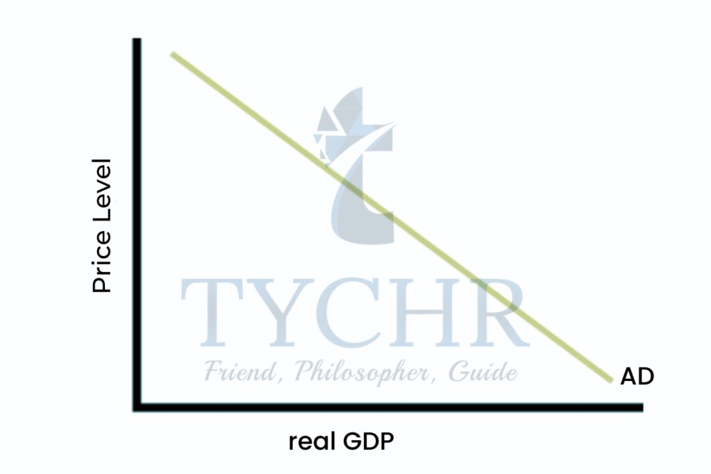
AD curve shows relationship between real GDP demanded & price level, ceteris paribus.

The negative slope is a result of:

• The wealth effect: Price level changes affect wealth (value of assets people own).
  • Upward movement along the AD curve if the price level increases. Real wealth value falls so people feel worse off.
  • Downward movement along the AD curve if price level decreases. More output is demanded because real wealth value increases.
• The interest rate effect: price level changes affect Interest rates.
  • Increase in price level -> increase demand for money to buy Items –>Increase in Interest rates -> cost of borrowing Increases -> decrease in consumer purchases
• The international trade effect: if domestic price levels increase out foreign price levels remain the same, exports become more expensive··> foreign buyers demand less. Domestic buyers buy more imports, causing a fall in net exports.
  The difference between micro- and macroeconomic demand/AD is that macroeconomic AD is about all possible buyers to buy the aggregate output.
  • Reasons for downward slopes differ: micro – diminishing marginal benefits.

DETERMINANTS OF AD (SHIFTS)

1. A rightward shift of AD curve – for any price level, a larger amount of real GDP demanded.
2. A leftward shift of AD curve- for any price level, a smaller amount of real GDP demanded.

Consumption spending changes

Consumer confidence – how optimist consumers are about the future

1. High confidence: rightward shift
2. Low confidence: leftward shift

Interest rate changes

1. Increase in interest rates results in lower consumption: leftward shift
2. Decrease in interest rates results in more consumption: rightward shift

Wealth changes

1. Increase in consumer wealth: rightward shift
2. Decrease in consumer wealth: leftward shift

Personal income tax changes

1. Increase in personal income tax: leftward shift
2. Decrease in personal income tax: rightward shift

Household indebtedness changes –  how much $ people owe from taking out loans

1. High levels of indebtedness: leftward shift due to people trying to pay back loans
2. Debt levels that are low: shift to the right

Spending on investments changes.

Changes in business confidence are the level of optimism businesses have regarding future sales.

1. High confidence: rightward shift
2. Low confidence: leftward shift

Interest rate changes

1. Increase in Interest rate: leftward shift
2. Decrease in Interest rates: rightward shift

Improvements in technology –

stimulate investment spending: rightward shift

Business tax changes

1. Increase in taxes: leftward shift
2. Decrease in taxes: rightward shift

Corporate indebtedness changes

1. High debt levels: leftward shift
2. Low debt levels: rightward shift

Legal/institutional changes – some economies don’t offer credit to small businesses

1. Increasing credit access: rightward shift

Government spending changes

Political priorities changes

1. Governments have expenditures. Increase in spending: rightward shift
2. Reduced spending: shift to the left

Changes in economic priorities: attempts to change AD

1. Government can use spending to influence aggregate demand.

Net export changes

National income abroad changes

• If a country’s national income increases, it will import more goods from another country, shifting that country’s AD curve to the right.

Exchange rate changes

• Country A’s currency price increase: leftward shift because less exports
  Country A’s currency price decreases: rightward shift because more exports

Trade protection changes

• Other countries set trade restrictions on imports. leftward shift because less exports

Changes in national income cannot cause AD curve shifts because the real GDP axis also represents national income.

Don’t confuse the wealth effect (resulting from price level change) with the factor that affects AD shifts (no price level changes).

Short-run aggregate supply & short run equilibrium in the AD-AS model

SHORT RUN AND LONG RUN

Short run in macroeconomics – period of time where prices are constant/inflexible and don’t change much, especially in labor costs.

• In terms of wages, there are contracts for wages over time periods.

Long run in macroeconomics – period of time where prices are flexible and changes with changes in the price level.

SHORT RUN AGGREGATE SUPPLY

Aggregate supply (AS) – total quantity of goods/ services produced in an economy over a time period at different price levels.
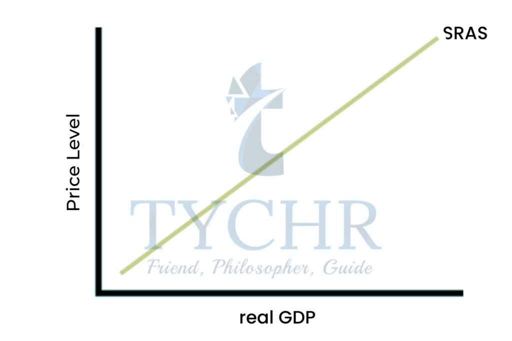
Short-run aggregate supply (SRAS) curve – when resource prices remain constant, the relationship between price level and real GDP is shown.

There is a positive slope because.

1. An increase in price level means output prices have increased but resource prices have not (short run), so production becomes more profitable.

SRAS CURVE SHlFTS

Wage changes (price level constant)

1.) If wages increase, cost of production rises: leftward shift2.) If wages decrease, cost of production decreases: rightward shift

Non-labor resource price changes

1.)If non-labor resource prices rise: leftward shift
2.)If non-labor resource prices decrease: rightward shift

Business tax changes – they are treated like costs of production

1.) increase in tax: leftward shift
2.) Decrease in tax: rightward shift

Subsidy changes

1.) Increase in subsidies: rightward shift
2.) Decrease in subsidies: leftward shift

Supply shocks

1.) Events that cause a decrease in output: leftward shift
2.) Events that cause increase in output: rightward shift

SHORT-RUN EQUILIBRIUM IN THE AD-AS MODEL

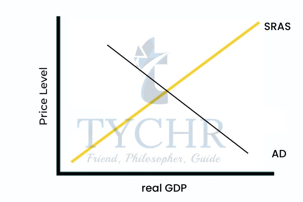
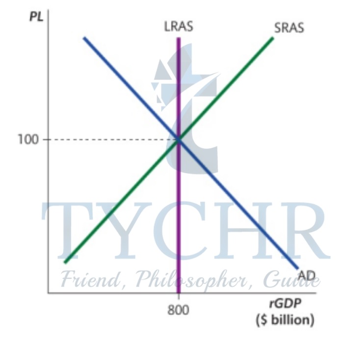
Equilibrium level of output (real GDP) is where AD intersects AS. In the short-run, it is where AD intersects SRAS.

In the above diagram, Ys is the equilibrium level of real GDP and Ple is the equilibrium price level.

The equilibrium leveI of real GDP can determine unemployment:

• increase in real GDP: decreased unemployment
• decrease in real GDP: increased unemployment

At PI1 excess real GDP supplied. At Pl2 excess real GDP demanded.

SHORT-RUN EQUILIBRIUM POSITIONS

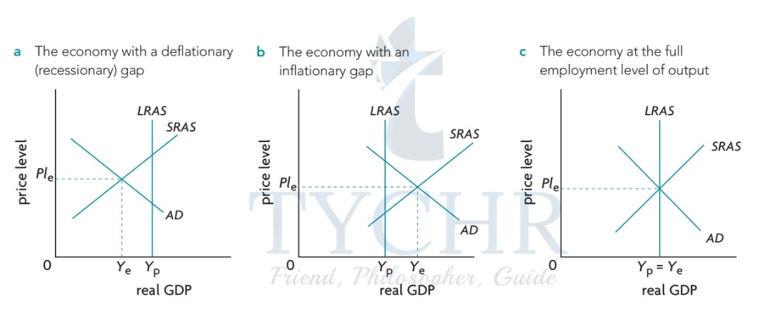
There are 3 types of short-run macroeconomic equilibrium positions, defined in relation to the economy’s potential output (Yp), which represents the level of real GDP where there is full employment.

Deflationary (recessionary) gap

• The potential GDP exceeds the real GDP.
• Unemployment greater than the natural rate.
• Not enough demand to produce potential GDP.
• Firms require less labor.

Inflationary gap

• Real GDP greater than potential GDP.
• Unemployment is less than the natural rate.
• Too much demand; firms produce more GDP.
• Firms need more labor 10 produce more output.

Full employment of real GDP

• Real GDP is equal to potential GDP.
• Unemployment equal to the natural rate.

IMPACTS OF CHANGES IN SHORT-RUN EQUILIBRIUM

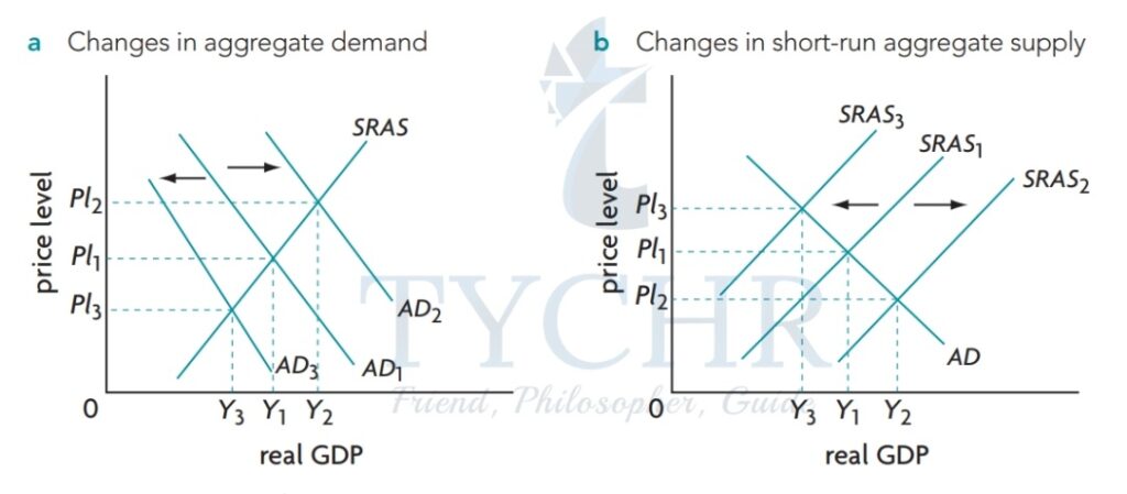
• If AD shifts from AD1 to AD2, there is an increase in price-level and real GDP. Can lead to a fall in unemployment.
• If there’s an AD decrease, there is a fall in real GDP and price level, and can lead to an increase in unemployment.
• If there is an increase in SRAS, there will be a higher real GDP, a lower price level, and lower unemployment.
  A leftward shift of SRAS will increase the price level, while the real output falls. Unemployment will increase.

AD OR SRAS SHIFTS AS CAUSES OF THE BUSINESS CYCLE

• In the CHANGES IN AD diagram the economy is at equilibrium.
  • If AD falls to AD2, a recessionary gap will form.
  • If AD moves to AD3, an inflationary gap will form.
• In the CHANGES IN SRAS diagram the economy is at equilibrium.
  • If SRAS falls to SRAS2, there will be an economic contraction. Real GDP will fall to Y2 and unemployment will increase. Price level will increase.
    • Different from recessionary gap from AD fall. Two problems, recession and a rising price level will occur (stagflation).
• If SRAS increases to SRAS3, real GDP increases and unemployment falls. There is a falling price level.
• Economists believe that AD changes are more important than AS changes.

Long run aggregate supply and LR equilibrium in monetarist/new classical model

MONETARIST/ NEW-CLASSICAL MODEL

1.) The monetarist/new classical model builds from 19th century classical economists. Key principles:

• Importance of price mechanism
• Concept of competitive market equilibrium
• Economy as harmonious system that tends towards full employment

2.) Monetarist approach to AS differs on short run and long run.

3.) The long run relationship is the long run aggregate supply (LRAS). The LRAS curve is vertical at Yp (potential GDP).

• In the long run, change in price level does not affect the quantity of real GDP.

4.) The LRAS curve is vertical because in the short run, if the price level increases when other inputs are constant, the quantity of output moves upward along the curve. However, in the long run the input prices increase by the same amount.

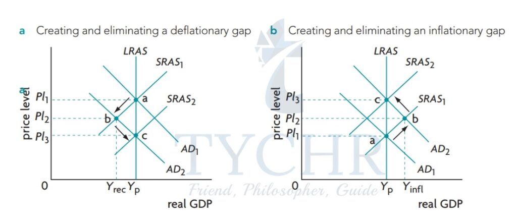
5.) In the long run, according to the monetary/new classical model output gaps cannot persist.

6.) In the figure to the right, a recessionary gap has formed because AD1 falls to AD2. However, in the long run the fall in price level is matched by decrease in resource prices which shifts the SRAS curve to the right. The gap has disappeared though the price level has fallen.

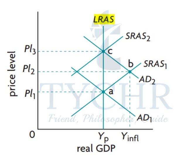
7.) In the lower figure, an inflationary gap has formed because AD2 to AD1. In the long run wages also increase, so SRAS curve shifts to the left resulting at point c. The gap disappeared but the price level increased.

8.) In the monetarist/new classical point of view, gaps are removed in the long run. The economy moves towards equilibrium. Changes in AD can affect real GDP only in the short run. In the long run the only impact of an AD change is the price level, so AD increase in the long run can be inflationary.

Aggregate Supply and Equilibrium in the Keynesian model

KEYNESIAN MODEL

• It bases ideas on John Maynard Keynes’ work. It showed that it is possible for economies to stay in the short run equilibrium for long periods of time.
• What if resource prices can’t fall? Asymmetry between wage changes.
  • Inflationary gaps: Unemployment lowers, price level rises, wages move upwards.
  • Recessionary gaps: Unemployment rises, but wages don’t fall as easily because of factors like contracts, minimum wages and union resistance.
• Keynesians also argue that the product prices don’t fall easily because firms won’t lower prices if wages don’t go down. Oligopolies fear price wars. Prices are not likely to fall during a recession.
• Economy gets stuck in the short run if prices don’t fall easily.

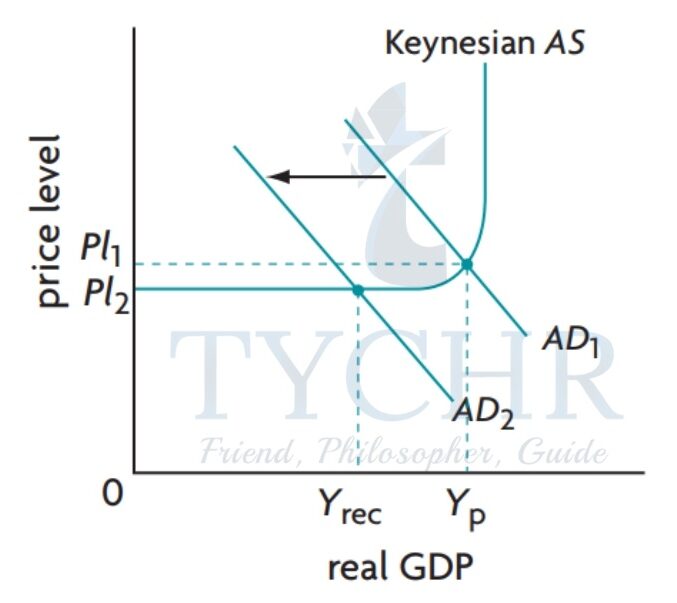
• Above figure is like the recessionary gap but if the price level cannot fall from PL1 then the economy will move to pt. D. If the price level drops to PL2, it might not be able to shift back to eliminate the gap.

• It suggests that the above SRAS curve looks like the Keynesian AS curve.
  • The economies are in a recessionary gap and the government needs to intervene.
• Keynesian aren’t saying that wages won’t fall at all, eventually they will begin to fall, but long recessions aren’t good for the economy.

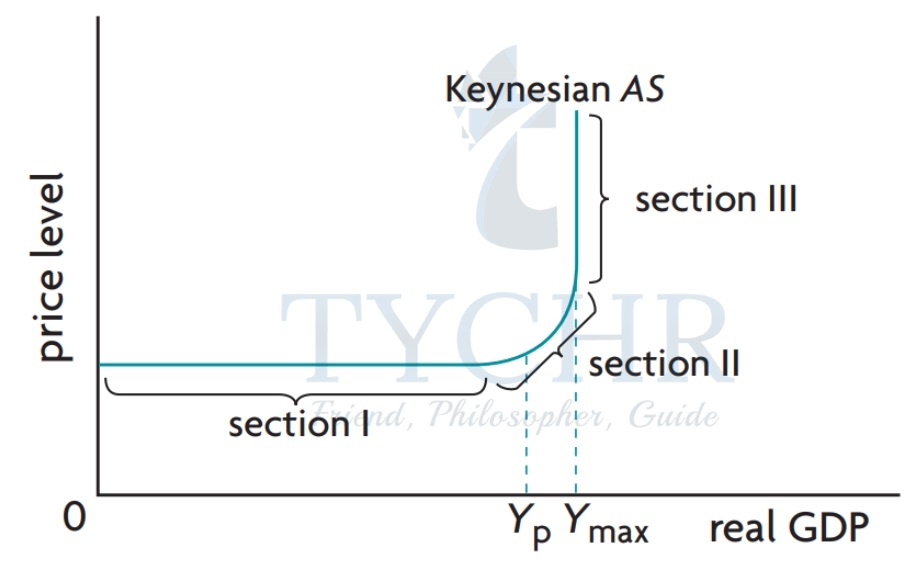
KEYNESIAN AS CURVE

It has 3 parts:-

Section I: Real GDP low, price level constant as GDP increases. Lots of unemployment in spare capacity.
Section II: Real GDP and price level increases but spare capacity soon decreases. Only way to increase output is to sell at a higher price. Full employment level.
Section III: AS curve becomes vertical, real GDP cannot increase and the price level increases rapidly.

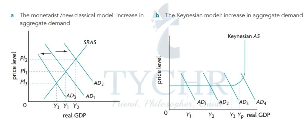
3 EQUILIBRIUM STATES OF KEYNESIAN MODEL

Recessionary gap – The AD curve (AD1) intersects at the horizontal section, less than the potential GDP.

Inflationary gap – The AD curve (AD3) intersects at the vertical section, greater than the potential GDP.

Full employment equilibrium – AD2 curve, which intersects the potential GDP YP.

These terms, inflationary and deflationary gaps are Keynesian concepts. Potential output and natural unemployment are monetarist concepts.

The Keynesian perspective says that recessionary gaps can happen for a long time, until the gov’t helps with specific ways to allow it to come out.

It is a short-run analysis and they don’t accept the idea that the economy can move into the long-run and that it tends to full employment equilibrium.

In the Keynesian model, AD increase doesn’t always cause a price level Increase. From a monetarist point of view, an increase in AD results in an increase in price level.

Shifting AS curves over the long term

INCREASE IN AS OVER LONG TERM

1.) These factors shift the AS curve to the right. Their opposites shift the curve to the left.

• Factors of production quantity increase: rightward
• Factor of production quality improvement: rightward
• Technology improvement: rightward
• Efficiency Improvement: rightward
  • Institutional changes
• Natural rate of unemployment reduction: rightward

2.) Rightward shifts correspond to long-term growth (increase in potential output). Short term economic growth does not cause this.

3.) In the monetarist/new classical model, factors that shift the LRAS curve shift the SRAS curve over the long term.

4.) Events with a temporary effect on aggregate supply can shift the SRAS curve temporarily without shifting the LRAS curve.

Illustrating monetarist/new classical & Keynesian models

The Keynesian Multiplier

It is the ratio of change in national income (real GDP) arising from a change in government spending.

Multiplier (K) = Change in real GDP / Initial change in expenditure
Note: If K>1, change in GDP > change in expenditure

Change in multiplier in terms of injections and leakages

Marginal Propensity to consume (MPC):- Change in consumption due to change in income.
Marginal Propensity to save (MPS):- Fraction of additional income saved.
Marginal Propensity to tax (MPT):- Fraction of additional income taxed.
Marginal Propensity to import (MPM):- Fraction of additional income spent on imported goods and services.

Note: Formula: MPC + MPS + MPT + MPM = 1
Multiplier = 1 / 1 – MPC or 1 / MPS + MPT + MPM
The value of the multiplier is given by 1 / 1 – MPC, which is equivalent to 1 / MPS + MPT + MPM. Therefore, if we know MPC, we can calculate the multiplier’s value.

Conclusion: Larger the MPC, the greater the multiplier. Smaller the leakages, greater the multiplier.

The multiplier aggregate demand and real GDP

Effect of multiplier on price level

The full effect of the multiplier can be experienced only when the price level is constant. If the price level is increasing, the greater the price level increases, the smaller is the size of the multiplier effect.

Aggregate demand and the multiplier : Keynesian cross model

Desired consumption and desired investment spending

Desired Consumption: It is the expenditure, consumer desires to make on final goods and services. It depends on consumer’s real income.

• In the figure below we can see :-
  • There is a direct relationship between consumption (C) and real income (Y). If C increases so does Y.
  • There is a 45o line between the 2 axes. This line represents all points of equality between the variables measured on the 2 axis.
  • At point ‘b’, C=Y. At pt. ‘a’, C>Y. At pt. ‘c’, C<Y.

Note: Consumption Function: It is the ‘C’ line, representing consumption spending. It has a constant slope, given by dC/dY.

This slope is known as Marginal Propensity to Consume (MPC), which means the change in consumption due to change in income.

• The shape of the consumption function depends on the ‘desired saving’.
  Y = C + S, Income = Desired consumption + Desired saving
• Negative Savings (C>Y): Income is used to buy necessities. (It means consumers are borrowing or using past savings).
• Positive savings (C<Y) :

Autonomous and Induced spending

Autonomous spending: Spending which is independent of income.
Induced Spending: Spending which is dependent on income.

Equilibrium level of Income and Output:-

In the figure below, Ye = Equilibrium point. At Y1 Consumption > real GDP produced. Hence, firm’s inventories are sold, thus providing firms with the signal to increase production causing real GDP to increase to Ye.
At Y2, Consumption < real GDP produced. Hence, the firm’s stock is lying idle, signaling a cut down on production, so real GDP falls to Ye.
Note: Equilibrium point is Ye where desired saving (leakages) = Desired investment (injection)

Adding Government (G) and Foreign sector (exports X- imports M or Xn =net exports)

G and Xn both are autonomous (independent of income).

Note: ‘X’ is an injection which increases desired spending. While ‘M’ is a leakage which reduces desired spending.
If X>M, spending increases. If X<M spending decreases.

Aggregate expenditure represents total desired spending (C+I+G+Xn) When aggregate expenditure = Real GDP, Economy is in equilibrium.

Relating aggregate expenditure to aggregate demand

Each point on the aggregate demand curve corresponds to a particular price level where the amount of output buyers want to buy is just that output that generates the spending needed to buy the output

The Keynesian cross model and output gaps

In the Keynesian cross model, equilibrium can occur at any level of output and there is nothing to guarantee that the equilibrium level of output will be the same as potential output. Recessionary (deflationary) gaps or inflationary gaps may persist indefinitely.

Recessionary gap (Ye < Yp): At Ye, there exists unemployment and recession. Actual equilibrium output is less than the potential output and unemployment > natural rate of unemployment.

Inflationary gap (Ye > Yp): At Ye, unemployment < natural rate of unemployment and actual output > potential output.

The Keynesian Multiplier

The multiplier is a Keynesian concept showing the power of increased spending to induce a larger increase in real GDP when the economy is in recession and is not experiencing upward pressure on the price level.

Relationship between multiplier and MPC: larger the MPC, larger the multiplier.

Note: MPC is the slope of the aggregate expenditure function (F), because larger the slope of F, larger the multiplier and steeper the aggregate expenditure function and vice versa.

When MPC = 0, multiplier (1/ 1-MPC) is 1.
Because MPC is 0, this indicates that all of the increased income is saved and that nothing is spent.