


Table of Contents
Unit 1: Number and Algebra
| Chapter Number | IB Points to Understand |
| 1.1 | Conducting mathematical operations with exponential numbers and expressing them in terms of a x (bk) where a ranges from 0 < a < 10. |
| 1.2 | Sequence- A sequence is a list of numbers that is written in a defined order, ascending or descending, following a specific rule.
Series- A series is the sum of all the terms in a sequence. A finite sequence has a fixed number of terms. An infinite sequence has an infinite number of terms. A term in a sequence is named using the notation 𝑎𝑛, where 𝑛 is the position of the term in the sequence. A term in a sequence is named using the notation 𝑎𝑛, where 𝑛 is the position of the term in the sequence. A sequence formed when each term after the first is found by adding a fixed non-zero number is called an arithmetic sequence. Adding up the terms of an arithmetic sequence gives us arithmetic series. |
| 1.3 | A sequence in which every term is obtained by multiplying or dividing a non-zero number with the preceding number is known as a geometric sequence.
When 𝑟 > 1, the sequence is diverging. A geometric series with 𝑟 < 1 and with infinite number of terms is called an infinite geometric series. |
| 1.4 | Applications of Geometric sequences and series:
|
| 1.5 | Exponential operations and laws
Logarithms and numerical evaluation of logarithms |
| 1.6 | Approximations are a value or quantity that is nearly but not exactly correct.
Percentage error expresses as a percentage the difference between an approximate or measured value and an exact or known value. Significant figures are used to express it to the required degree of accuracy, starting from the first non-zero digit. Estimations are rough calculations of the value, number, quantity, or extent of something. |
| 1.7 | Annuities are a sequence of equal payments made at regular time intervals and amortisation determines sequence of payments. |
| 1.8 | Using technology to solve:
|
| 1.9 (HL) | Laws of logarithms:
logaxy = logax + logay logaxy = logax … logay logaxm = mlogax for a, x, y > 0 |
| 1.10 (HL) | Simplifying expressions, both numerically and algebraically, involving rational exponents. |
| 1.11 (HL) | The sum of infinite geometric sequences. |
| 1.12 (HL) | Real numbers are simply the combination of rational and irrational numbers, in the number system.
Complex numbers cannot be represented on the number line, but are analytic solutions to equations whose solutions are not real numbers. These complex numbers have an imaginary unit. A number that is expressed in terms of the square root of a negative number is called an imaginary number. |
| 1.13 (HL) | |z| is the modulus of the complex number and the argument of z is defined as the angle between the positive real axis and the line from origin to z.
The polar form of a complex number z = a + bi is z = r(cosθ + isinθ) Euler’s formula is the statement that 𝑒𝑖𝜃 = cos(𝜃) + isin(𝜃) DeMoivre’s Theorem states that zn = (r𝑒𝑖𝜃)n = rn 𝑒𝑖 𝑛𝜃 Forming and converting between Cartesian, polar and exponential forms Polar or exponential forms – calculating products, quotients and integer powers Vector addition and subtraction(Geometric interpretation of complex numbers) |
| 1.14 (HL) | Matrix refers to an ordered rectangular arrangement of numbers which are either real or complex or functions.
Types of matrices: Row, Column, Square, Diagonal, Zero, Upper Triangular and Lower Triangular Adding and subtracting matrices Addition of matrices is commutative which means A+B = B+A Addition of matrices is associative which means A+(B+C) = (A+B)+C whereas subtraction is neither. Scalar multiplication refers to the product of a real number and a matrix. Multiplication of matrices is non-commutative which means A*B ≠ B*A Multiplication of matrices is associative which means A*(B*C) = (A*B)*C If the determinant of the matrix ≠ 0, then the inverse of the matrix exists. |
| 1.15 (HL) | An eigenvector of a matrix A is a vector whose product when multiplied by the matrix is a scalar multiple of itself. The corresponding multiplier is often denoted as 𝜆 and referred to as an eigenvalue.
A·v = λ·v An n × n matrix A is diagonalizable if it is similar to a diagonal matrix: that is, if there exists an invertible n × n matrix P and a diagonal matrix The method we can use to find the matrix representing a transformation is given by the Matrix Basis theorem. |
Unit 2: Functions
| Chapter Number | IB Points to Understand |
| 2.1 | Different forms of the equation of a straight line. Gradient; intercepts.
Lines with gradients m1 and m2 Parallel lines m1 = m2. Perpendicular lines m1 × m2 = … 1. |
| 2.2 | A function is a relation from a set of inputs to a set of possible outputs where each input is related to exactly one output.
The domain of a function is the complete set of possible values of the independent variable. We determine the domain of each function by looking for those values of the independent variable The range of a function is the complete set of all possible resulting values of the dependent variable, after we have substituted the domain. An inverse function or an anti-function is defined as a function, which can reverse into another function. The method of calculating an inverse is swapping of coordinates x and y. |
| 2.3 | The graph of a function f is the set of all points in the plane of the form (x, f(x)). We could also define the graph of f to be the graph of the equation y = f(x).
Sketching and drawing graphs with given equations |
| 2.4 | The graph of a function f is the set of all points in the plane of the form (x, f(x)). We could also define the graph of f to be the graph of the equation y = f(x).
Determination of key features of a graph – maximum and minimum values, root values, intercepts, horizontal and vertical asymptotes, vertices of a given graph |
| 2.5 | Linear Function: A linear function f(x) = mx+c where m and c are constants, represents a context with a constant rate of change.
Quadratic models. f x = ax2 + bx + c ; vertex, zeros and roots, intercepts on the x-axis and y -axis. a ≠ 0. Axis of symmetry, Exponential growth and decay models. f (x) = kax + c f(x)=ka…x+c (fora>0) f (x) = kerx + c Equation of a horizontal asymptote. Direct/inverse variation: fx=axn, n∈Z The y-axis is a vertical asymptote when n < 0. Cubic models: f x =ax3+bx2+cx+d. Sinusoidal models: f x = asin(bx)+d, |
| 2.6 | Modelling
Understanding and selecting or identifying models, parameters, |
| 2.7 | Composite functions in context. The notation (f ∘ g)(x) = f(g(x)).
Inverse function f …1, including domain restriction. Finding an inverse function. |
| 2.8 | Transformations of graphs
Translations: y = f (x) + b ;y = f (x … a). Reflections: in the x axis y = … f (x), and in the y axis y = f ( … x). Vertical stretch with scale factor p: y = p f (x). Horizontal stretch with scale factor 1q : y = f (qx) Composite transformations |
| 2.9 (HL) | Exponential model arise in situations where the rate of change is a constant factor.
Exponential decay and be used to model radioactive decay and depreciation. Exponential decay models of this form can model sales or learning curves where there is an upper limit. The logarithmic model has a period of rapid increase, followed by a period where the growth slows, but the growth continues to increase without bound. Piecewise functions: A piecewise function is a function where more than one formula is used to define the output. Any motion that repeats itself in a fixed time period is considered periodic motion and can be modelled by a sinusoidal function. The logistics model begins with a slow growth, followed by a period of moderate growth, and then back to a period of slow growth. |
| 2.10 (HL) | Scaling very large or small numbers using logarithms.
Linearizing data using logarithms to determine if the data has an exponential or a power relationship using best-fit straight lines to determine parameters Interpretation of log-log and semi-log graphs. |
Unit 3: Geometry and Trigonometry
| Chapter Number | IB Points to Understand |
| 3.1 | Given the cartesian coordinates A(x1 , y1) and B(x2 , y2) the distance between A and B is given by:
AB = √(𝒙𝟐 − 𝒙𝟏)𝟐 + (𝒚𝟐 − 𝒚𝟏)𝟐 Lines and Intersections: Coincident lines, Parallel lines, Intersecting Lines If two lines are perpendicular to each other, one is said to be normal to the other at the point of intersection. Given the cartesian coordinates A (x1, y1, z1) and B (x2, y2, z2) the distance between A and B is given by: AB = √(𝒙𝟐 − 𝒙𝟏)𝟐 + (𝒚𝟐 − 𝒚𝟏)𝟐 + (𝒛𝟐 − 𝒛𝟏)𝟐 Angles of rotation are formed in the coordinate plane between the positive x-axis (initial side) and a ray Formula for surface area and volume of geometric solids |
| 3.2 | Use of sine, cosine and tangent ratios to find the sides and angles of right-angled triangles.
Sine rule and cosine rule Area of a triangle = |
| 3.3 | Equilateral: “equal”-lateral, so they have all equal sides.
Isosceles: means “equal legs”, they have two equal “sides” joined by an “odd” side. Scalene: means “uneven” or “odd”, so no equal sides. The term angle of elevation denotes the angle from horizontal upward to an object. The term angle of depression denotes the angle from horizontal downward to an object. Pythagoras theorem states that in a right-angled triangle, the square of the hypotenuse side is equal to the sum of squares of the other two sides |
| 3.4 | Length of Arc
Area of the sector Note: Measurements in radians not part of SL |
| 3.5 | Equations of perpendicular bisectors. |
| 3.6 | Voronoi diagram is a partition of a plane into regions close to each of a given set of objects and its real-life application of the toxic waste dump issue.
Nearest neighbor interpolation |
| 3.7 (HL) | Radian measures may be expressed as exact multiples of π, or decimals.
Using radians to calculate area of sector, length of arc. |
| 3.8 (HL) | Definition of tanθ as sinθ/cosθ
The Pythagorean identity: cos2θ + sin2θ = 1 Ambiguous case of the sine rule Solving trigonometric equations graphically within a finite interval (sinusoidal models) |
| 3.9 (HL) | The method we can use to find the matrix representing a transformation is given by the Matrix Basis theorem.
Geometric transformations with matrices – translations, rotations, reflections, horizontal and vertical stretching and enlargements Producing fractals using iterative techniques with compositions of the above transformations |
| 3.10 (HL) | Scalar is a quantity which only has magnitude, but a vector has both magnitude and direction.
Unit vectors have a magnitude of 1. They are represented by 𝒗̂ = v/|v| where |v| represents the magnitude of vector v. The position vector of a point P, with coordinates (x, y, z), is the vector 𝑟⃗ with initial point on the origin and terminal point on P. Rescaling and normalizing vectors |
| 3.11 (HL) | When a vector is represented graphically, its magnitude is represented by the length of an arrow and its direction is represented by the direction of the arrow. |
| 3.12 (HL) | The trajectory of a moving point can be determined at every moment t by an expression for the position vector of the point as a function of time
Vectors in kinematics Modeling linear motion in 2D and 3D with constant velocity |
| 3.13 (HL) | Scalar product or dot product is an algebraic operation that takes two equal-length sequences of numbers and returns a single number.
Vector product or cross product is a binary operation on two vectors in three-dimensional space. Angles between two vectors can also be found using dot product and cross product. Geometric interpretation of – (Area of parallelogram) Components of vectors |
| 3.14 (HL) | A graph is defined as a set of vertices and a set of edges. A vertex represents an object. An edge joins two vertices.
A graph G is said to be connected if there exists a path between every pair of vertices. Varieties of graphs:
|
| 3.15 (HL) | For a graph with |V| vertices, an adjacency matrix is a ∣V∣×∣V∣ matrix of 0s and 1s, where the entry in row i and column j is 1 if and only if the edge (i, j) is in the graph.
Weighted adjacency tables Transition matrix construction |
| 3.16 (HL) | The cost of the spanning tree is the sum of the weights of all the edges in the tree.
Minimum spanning tree has direct application in the design of networks. Kruskal’s Algorithm builds the spanning tree by adding edges one by one into a growing spanning tree. In Prim’s Algorithm we grow the spanning tree from a starting position. A connected graph G is Eulerian if there exists a closed trail containing every edge of G. Such a trail is an Eulerian trail. In graph theory, an Euler cycle in a connected, weighted graph is called the Chinese Postman problem. A path is a walk which does not pass through any vertex more than once. A cycle is a walk that begins and ends at the same vertex A Hamiltonian path or cycle is a path or cycle which passes through all the vertices in a graph. The classical traveling salesman problem (TSP) is to find the Hamiltonian cycle of least weight in a complete weighted graph. An upper bound can be found using the nearest neighbour algorithm Lower bounds can be found by using spanning trees. |

Unit 4: Statistics and Probability 
| Chapter Number | IB Points to Understand |
| 4.1 | Population, samples, random samples, discrete and continuous data
Understanding and determining reliability and bias of data in sampling Interpretation of outliers Effectiveness of various sampling techniques(simple random, convenience, systematic, quota and stratified) |
| 4.2 | A histogram is very similar to a bar chart but bar charts are used for graphing qualitative data and histograms are used for quantitative data.
A box and whisker plot—also called a box plot—displays the five-number summary of a set of data. The cumulative frequency of a set of data or class intervals of a frequency table is the sum of the frequencies of the data up to a required level. Types of correlation Interpolation is where we find a value inside our set of data points. Extrapolation is where we find a value outside our set of data points |
| 4.3 | A measure of central tendency is a summary statistic that represents the center point or typical value of a dataset.
The mean is the arithmetic average. The mode is the value that occurs most frequently in a set of data. The median is the middle data value when the data values are arranged in order of size. Range is found by subtracting the smallest number from the largest number. Standard deviation gives an idea how the values are related to the mean. Variance is given by 𝜎2 Measure of dispersion of data Quartiles of discrete data |
| 4.4 | Linear correlation of bivariate data
Pearson’s product-moment correlation and its coefficient r – only applicable in linear relationships Scatter diagrams Equation of regression line of y on x, using it in prediction and interpretation of its parameters, a and b, in the linear regression y = ax + b. |
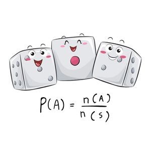
| 4.5 | Experiment: A process by which you obtain an observation.
Trials: Repeating an experiment a number of times. Outcome: A possible result of an experiment. Event: An outcome or set of outcomes. Sample space: The set of all possible outcomes of an experiment, always denoted by U. |
| 4.6 | A venn diagram represents mathematical or logical sets pictorially as circles or closed curves within an enclosing rectangle (the universal set), common elements of the sets being represented by intersections of the circles.
To solve problems involving independent events, it is often helpful to draw a tree diagram. Sample space is a term used in mathematics to mean all possible outcomes. The conditional probability (which is basically Bayes’ theorem) of an event B is the probability that the event will occur given the knowledge that an event A has already occurred. Independent events |
| 4.7 | They can be discrete or continuous. All the probability distributions that we are going to discuss come under discrete random variables (DRV).
The variance of a discrete random variable measures the spread or the variability of the distribution and is denoted by 𝜎2=∑𝑛 (𝑥−𝜇)2𝑃(X=xi) If a random variable takes all possible values between two limits or if it represents a real number then the random variable is called a continuous random variable. Expected value – E(X) Applications of discrete data |
| 4.8 | Binomial Distribution and calculation of its mean and variance |
| 4.9 | A normal distribution is a binomial distribution for a very large n and the probability of success is close to half.
Normal probability Inverse normal calculations |
| 4.10 | The Spearman’s Rank Correlation Coefficient is used to discover the strength of a link between two sets of data. The notation used is rs. |
| 4.11 | A statistical hypothesis is an assumption about a population parameter.
Null and alternative hypothesis The p-value is the probability of observing a sample statistic as extreme as the test statistic. Contingency tables (also called crosstabs or two-way tables) are used in statistics to summarize the relationship between several categorical variables. A test of a statistical hypothesis, where the region of rejection is on only one side of the sampling distribution, is called a one-tailed test and a test of a statistical hypothesis, where the region of rejection is on both sides of the sampling distribution, is called a two-tailed test. The t-test is a statistical test which is widely used to compare the mean of two groups of samples. One-sample t-test is used to compare the mean of a population to a specified theoretical mean (μ). Independent (or unpaired two sample) t-test is used to compare the means of two unrelated groups of samples Paired sample t-test: To compare the means of the two paired sets of data, the differences between all pairs must be, first, calculated. |
| 4.12 (HL) | Categorising numerical data in a χ2 table and justifying the choice of categorisation.
Choosing an appropriate number of degrees of freedom when estimating parameters from data when carrying out the χ2 goodness of fit test. Definition of reliability and validity. Reliability tests Validity tests |
| 4.13 (HL) | Non-linear regression and least squares regression curves(with technology)
gives the proportion of variability in the second variable accounted for by the chosen model. Sum of square residuals to determine the fit for a model The connection between the coefficient of determination and the Pearson’s product moment correlation coefficient for linear models. |
| 4.14 (HL) | Linear transformation of single random variable
Expected value of linear combinations of n random variables. Variance of linear combinations of n independent random variables Unbiased estimates |
| 4.15 (HL) | Normal distribution of n independent normal random variables
Central Linear theorem |
| 4.16 (HL) | Confidence intervals for the mean of a normal population. |
| 4.17 (HL) | Poisson distribution gives the probability of happening of the number of events occurring in a fixed interval of time, space or any other parameter with a known average. Mean and variance of poisson distribution
Sum of two separate Poisson distributions |
| 4.18 (HL) | To hypothesis test with the binomial distribution, we must calculate the probability, p, of the observed event and any more extreme event happening.
Testing hypotheses with the Poisson distribution is very similar to testing them with the binomial distribution. Type I error. A Type I error occurs when the researcher rejects a null hypothesis when it is true. Type II error. A Type II error occurs when the researcher fails to reject a null hypothesis that is false. |
| 4.19 (HL) | The transition matrix A associated to a directed graph is defined as follows. If there is an edge from i to j and the outdegree of vertex i is di, then on column i and row j we put 1/di.
A Markov chain is a mathematical system that experiences transitions from one state to another according to certain probabilistic rules. Initial state probability matrices Steady state and long-term probabilities using linear equation systems or transition matrices |
Unit 5: Calculus

| Chapter Number | IB Points to Understand |
| 5.1 | Suppose we have a function f(x). The value, a function attains, as the variable x approaches a particular value, say a, i.e., x → a is called its limit. |
| 5.2 | A function is increasing on an interval if for any x1 and x2 in the interval then, x1 < x2 implies f(x1) < f(x2)
A function is decreasing on an interval if for any x1 and x2 in the interval then, x1 < x2 implies f(x1) > f(x2) An Inflection Point is where a curve changes from Concave upward to Concave downward or vice versa. |
| 5.3 | The derivative of a function f(x) at any point ‘a’ in its domain is given by: limh->0 [f(a+h) – f(a)]/h |
| 5.4 | A tangent to a curve is a line that touches the curve at one point and has the same slope as the curve at that point.
A normal to a curve is a line perpendicular to a tangent to the curve. |
| 5.5 | Given a function, f(x), an anti-derivative of f(x) is any function F(x) such that F′(x) = f(x)
If F(x) is any anti-derivative of f(x) then the most general antiderivative of f(x) is called an indefinite integral and denoted by ∫ 𝑓(𝑥) 𝑑𝑥 = F(x) + c |
| 5.6 | Formation and Solution of given f(x)
Local minimum and maximum To find absolute maximum or minimum we need to find local extrema and then compare them to see which one is the greatest or least value for the entire domain of f(x). |
| 5.7 | In optimization problems we are looking for the largest value or the smallest value that a function can take. Here we will be looking for the largest or smallest value of a function subject to some kind of constraint. Some examples of where it is applied are profit maximisation and cost minimisation. |
| 5.8 | The area problem will give us one of the interpretations of a definite integral and it will lead us to the definition of the definite integral.
Given a function f(x) that is continuous on the interval [a,b] we divide the interval into n sub- intervals of equal width, Δx, and from each interval choose a point, xi. Using substitution with definite integral Midpoint and trapezoidal rule |
| 5.9 (HL) | Trigonometric, logarithmic and exponential equations and their derivatives
The chain rule states that the derivative of f(g(x)) is f'(g(x))⋅g'(x). Product Rule: If the two functions f(x) and g(x) are differentiable then the product is differentiable and (f(x)g(x))′ = f′(x)g(x) + f(x)g′(x) If the two functions f(x)f(x) and g(x)g(x) are differentiable (i.e. the derivative exist) then the quotient is differentiable Related rates of change |
| 5.10 (HL) | Second derivative of an equation
Suppose f(x) is a function of x that is twice differentiable at a stationary point x0. 1. If f’’(x0) > 0, then f has a local minimum at x0. 2. If f’’(x0) < 0, then f has a local maximum at x0. |
| 5.11 (HL) | Definite and indefinite integration
Integration by substitution |
| 5.12 (HL) | When calculating the area between a curve and the x-axis, you should carry out separate calculations for the parts of the curve above the axis, and the parts of the curve below the axis.
A similar technique to the one we have just used can also be employed to find the areas sandwiched between curves. To get a solid of revolution we start out with a function, y=f(x), on an interval [a, b]. The volume formula stays the same as the method of rings but the area differs. |
| 5.13 (HL) | Kinematics and problems of kinematics that utilise displacement s, velocity v and acceleration a. |
| 5.14 (HL) | Modelling differential equations in relation to a real-life scenario or given environment
A differential equation is an equation that contains a derivative. A separable differential equation is any differential equation that we can write in the following form: N(y) 𝑑𝑦 = M(x) |
| 5.15 (HL) | Slope fields are visual representations of differential equations of the form dy/dx = f(x, y). |
| 5.16 (HL) | After approximations and substitutions Euler’s formula is given by: yn = yn-1 + h f(tn-1, yn-1).
Producing and devising the numerical solutions of coupled systems |
| 5.17 (HL) | Phase portrait for the solutions of coupled differential equations of the form:
● dx/dt = ax + by ● dy/dt = cx + dy
Distinct, real, complex and imaginary Eigen values and analysing the future paths produced due to them Identifying equilibrium points, stable populations and saddle points with the creation and assistance trajectories and phase portraits |
| 5.18 (HL) | Euler’s method for solving second derivatives [d2x /dt2 = f (x, dx/dt , t)] |