Module 3.1: Research Methodology
What will you learn in this section?
- Research methodology: quantitative and qualitative methods
- Types of quantitative research: experimental, correlational, descriptive
- Types of qualitative research
- Qualitative versus quantitative comparison
- Sampling, credibility, generalizability and bias in research
Research methodology: quantitative and qualitative methods
- All research methods used in psychology can be categorized as either quantitative or qualitative. Data in quantitative research comes in the form of numbers.
- The goal of quantitative research is usually to arrive at numerically expressed regularities that characterize the behavior of large groups of individuals (i.e. universal laws).This is much like the aim of the natural sciences in which it has been the ideal for a long time to have a set of simple rules that describe the behavior of all material objects throughout the universe (think about laws of gravity in classic Newtonian physics, for example). In philosophy of science such orientation on deriving universal laws is called the nomothetic approach.
- Quantitative research operates with variables Any characteristic that can be objectively registered and quantified is a variable, which means “something that can take on varying values”. Since psychology deals with a lot of “internal” characteristics that are not directly observable, they need to be operationalized first. For this reason, there’s an important distinction between constructs and operationalizations.
- A construct is any theoretically defined variable, for example, violence, aggression, attraction, memory, attention, love, anxiety. To define a construct, you give it a definition which delineates it from other similar (and dissimilar) constructs. Such definitions are based on theories. As a rule constructs cannot be directly observed: they are called constructs for a reason—we have “constructed” them based on theory.
- To enable research, constructs need to be operationalized. Operationalization of a construct means expressing it in terms of observable behavior. For example, to operationalize verbal aggression, you might look at “number of abusive comments per hour” or “number of swear words per 100 words in most recent Facebook posts.”
- To operationalize anxiety, you can look at self-report scores on an anxiety questionnaire, levels of cortisol (the stress hormone) in your bloodstream, or weight loss. As you can see, there are usually several ways a construct can be operationalized; the researcher needs to use creativity in designing a good operationalization that captures the essence of the construct while being directly observable and reliably measurable.
Quantitative research
Quantitative research is of three types
1) Experimental studies:
- The experiment in its simplest form includes
a)independent variable (IV) :- The IV is the one manipulated by the researcher
b)one dependent variable (DV): DV is expected to change as IV changes.
c)while the other potentially important variables are controlled. - For example, if you want to study the effect of psychotherapy on depression, you can randomly divide participants into two groups:
a)the experimental group will receive psychotherapy while
b)the control group will not. - After a while, you can measure the level of depression by conducting a standardized clinical interview (diagnosis) with each of them. In this case, the IV is psychotherapy. You manipulate the IV by changing its value: yes or no.
- DV is depression; it is operationalized through a standardized diagnostic procedure. If the DV differs in two groups, you can conclude that the change in IV “caused” the change in DV.This is why experiment is the only method that allows us to infer cause and effect.
2)Correlational studies.
- Correlational studies differ from experiments in that the researcher does not manipulate any variables (there are no IVs or DVs). The relationship between variables is measured and quantified.
- For example, to find out if there is any relationship between violent behavior among adolescents and the amount of time they spend watching violent television programs, you can recruit a sample of adolescents and measure their violent behavior (by self-report, peer assessment, or even observation in natural settings) and average number of hours per day spent watching violent television programs.
- You can then correlate the two variables using a formula. Suppose you obtained a large positive correlation. This means that there is a trend in the data: the more time a teen spends watching violent shows, the more violent he is.
- However, cause and effect cannot be inferred from correlational studies. Since you did not manipulate one of the variables, you do not know the direction of the effect. It could be that watching violence influences violent behavior (that would probably be the most popular, intuitive assumption). However, it is also possible that teenagers who behave violently choose to watch violent television programs. Or there may even be a third variable (such as low self-esteem) that influences both violent behavior and viewing violence on television.
What you observe “on the surface” is just that – “correlation”, the fact that one variable changes as the other changes.
3)Descriptive studies
- In descriptive studies, relationships between variables are not examined and variables are approached separately.
- An example of a descriptive quantitative study might be a public opinion poll. We ask questions (eg, “Do you support the current policies of the president?”) and are interested in the distribution of responses to that particular question. Descriptive studies are often used in sociology and are sometimes used in psychology
Before you “dive deep” into the specs, do extensive research on the phenomenon.
Qualitative research
- Different is qualitative research. The in-depth investigation of a specific phenomenon is its primary focus. “Depth” refers to entering the realm of human experience, interpretation, and meaning beyond what can be objectively measured and quantified.
- Qualitative research uses such data collection methods as interviews or observations. Data comes in the form of texts: interview transcripts, observation notes, and so on. Data interpretation involves a degree of subjectivity, but the analysis is deeper than we can usually achieve with quantitative approaches. In the philosophy of science, such an orientation towards an in-depth analysis of a specific case or phenomenon (without trying to derive universally applicable laws) is called the idiographic approach.
Parameter | Quantitative research | Qualitative research |
Purpose | Nomothetic approach: derive universally applicable laws | Idiographic approach: in-depth understanding of a specific case or phenomenon |
Data | Numbers | Texts |
Focus | Behavioral manifestations (operationalizations) | Human experiences, interpretations meanings |
Objectivity | More objective (the researcher is discarded from the studied reality) | More subjective (the researcher is included in the studied reality) |
Sampling, credibility, generalizability and bias in research
- Sampling, credibility, generalizability, and bias are some of the characteristics used to describe a research study and assess its quality. These characteristics are universal to the social sciences, but quantitative and qualitative researchers may approach them very differently, sometimes even with vastly different sets of terms to express the same ideas. So it’s important that you understand both of these umbrella terms and how they are broken down in quantitative versus qualitative research.
Quantitative research | Qualitative research | ||
Overarching concepts | Experimental studies | Correlational studies | |
Sampling | Random Stratified Self- selected Opportunity | Same | Quota sampling Purposive sampling Theoretical sampling Snowball sampling Convenience sampling |
Generalizability | External validity:
| Population validity Construct validity | Sample-to-population generalization Case-to-case generalization Theoretical generalization |
Credibility | Internal validity: to what extent is the DV influenced by the IV and not by some other variable? Controlling for confounding variables: removing or keeping constant under all conditions | No special term used: “validity” and “credibility” can be used interchangeably If no biases occur the credibility will be high | Credibility = trustworthiness. What’s the limit the findings leave on an impact on reality? Triangulation Establishing a rapport Iterative questioning Reflexivity Credibility checks Thick descriptions |
Bias | Threats to internal validity: –
| At the level of variable measurement: depends on the method of measurement On the level of interpretation of findings:
| Participant bias-
Researcher bias: – Confirmation bias
|
Module 3.2: Quantitative research: the experiment
What will you learn in this section?
- Confounding variables
- Types of experiment
- Sampling in the experiment
- Random sampling
- Stratified sampling
- Opportunity sampling
- Self-selected sampling
- Experimental designs
- Independent measures design
- Matched pairs design; matching variable
- Repeated measures design; order effects; counterbalancing
- Credibility and generalizability in the experiment: types of validity
- Construct validity
- Internal validity
- External validity: population and ecological
Confounding variables
- Variables that can potentially confound the relationship between IV and DV (like Z in the above example) are called confounding variables. They contribute to bias. These variables need to be controlled, either by eliminating them or keeping them constant across all participant groups, so that they do not affect the comparison.
- For example, imagine that you manipulate X and observe the resulting changes in Y. However, every time you manipulate X, you also inadvertently change Z. In fact, it is Z that causes Y to change, but you mistakenly conclude that X (your IV) is the cause of Y , thereby incorrectly confirming your hypothesis. If this sounds too abstract, consider the following example: X is sleep deprivation (which you manipulate by waking up one group of participants every 15 minutes while they are asleep while a control group sleeps normally) and Y is memory performance (which you measure). a simple memory test in the morning). Without realizing that this may be an important factor, you let the control group sleep at home while the experimental group sleeps in the lab under the supervision of the experimenter. So
There is another variable, the Z variable: stress caused by an unfamiliar environment. It could be that in this experiment it was the unfamiliar environment (Z) that caused the reduction in memory performance (Y) rather than the sleep deprivation (X).
Types of experiment
- Laboratory experiments
- Laboratory experiments are performed in a controlled environment. using standardized procedures, Truth participants are randomly allocated to experimental groups.
- In a real environment, field experiments are carried out. The IV is manipulated by the researcher, but the participants remain in their natural surroundings. many extraneous variables cannot be controlled. The strength of eld experiments is the higher ecological validity compared to experiments in the laboratory. A limitation is less control over potentially confounding variables, thus lower internal validity. An example of an old experiment is Piliavin, Rodin, and Piliavin’s (1969) subway study, in which researchers simulated a collapse in a subway train and watched to see if other passengers came to help. To manipulate the IV, some researchers carried a cane (cane condition), while others carried a bottle (drunk condition).
Advantages And Weaknesses of Laboratory experiments
Advantages of laboratory experiments | Weaknesses of laboratory experiments |
|
|
Sampling
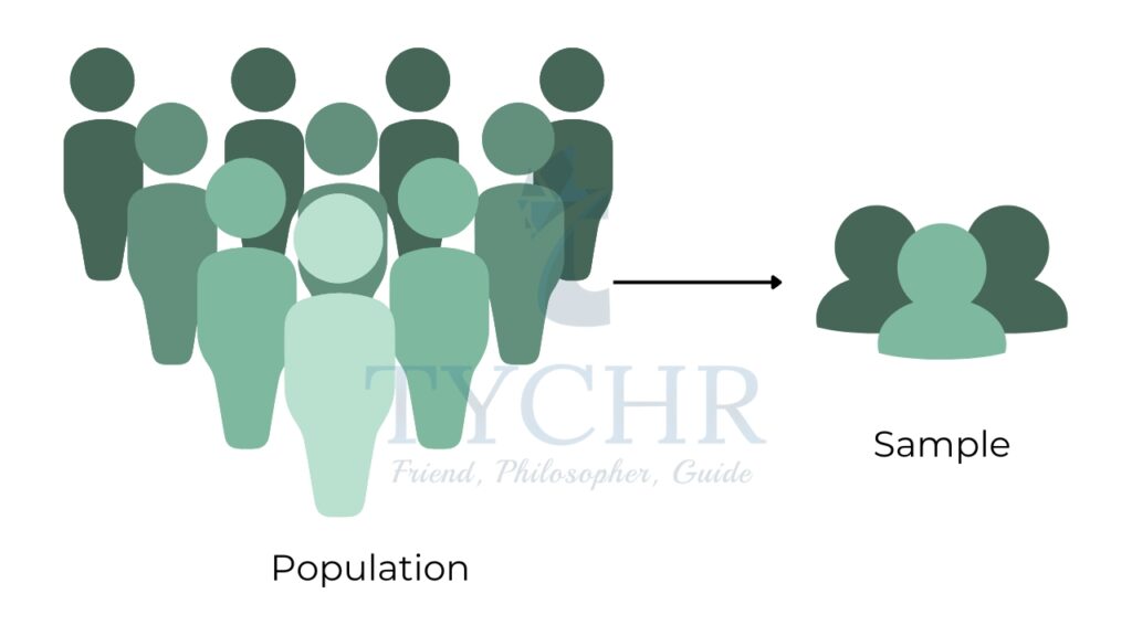
- A population is all of something, for example all the grains of sand on a breach. Researchers generally do not have the means to test whole populations, so they test a sample (part of population}. Ideally a sample is representative (contains the same characteristics as the population. population from which it was taken) and the term target population is used to indicate the group of people the results are targeted at. Psychologists use several sampling techniques, each with strengths and weaknesses.

Random sampling
- Each member of the population has an equal chance of being chosen through random sampling.One way to achieve this is to place all names from the target population in a container and draw out the required sample number, while computer programs are also used to generate random lists. This results in a sample selected in an unbiased fashion.
Strengths of random sampling | Weaknesses of random sampling |
|
|
Opportunity sampling
- Opportunity sampling involves selecting participants who are available and willing to take part; for example, asking people in the street who are passing. Sears (1986) found that 75 percent of university research studies use undergraduates as participants I simply for the sake of convenience.
Strengths of Opportunity sampling | Weaknesses of Opportunity sampling |
|
|
Volunteer (self-selected) sampling
- Volunteer or self-selected sampling involves people volunteering to participate. They select themselves as participants often by replying to adverts.
Strengths of Volunteer sampling | Weaknesses of Volunteer sampling |
|
|
Stratified sampling
- This method relies more on theory. First, you choose the essential traits that the sample needs to have. Then, you look at how these characteristics are distributed in the target population (you can use statistical data from various agencies for this). After that, you recruit your participants in a way that keeps the sample’s proportions the same as the population’s.For example, imagine that your target population is all students at your school. The characteristics you decide are important to the goal of study are age (elementary school, middle school, high school) and grade point average — GPA (low, average, high).
- You study school records to find the distribution of students in these categories For a stratified sample, you need to ensure that your sample has equal proportions. For each cell of this table, you can either randomly sample or use other approaches. In any case, stratified sampling is special in that it is based on theory and provides
that the theoretically determined basic characteristics of the population are fairly and evenly represented in the sample. This may be an ideal choice when you are certain of the baseline characteristics of the participants and when available sample sizes are not large
Experimental designs
- There are three main types of experimental design: the repeated measures design. The independent groups design and the matched pairs design.
Independent groups design
- In independent groups design [IGD] uses different participants in each of the experimental conditions, so that each participant only does one condition (either the experimental or control condition). Different participants are therefore being tested against each other.
Strengths of ( IGD )sampling | Weaknesses of (IGD )sampling |
|
|
Repeated measures design
- In a repeated measures design (RMDJ each participant is tested in all conditions of an experiment. Participants are therefore being tested against themselves.
Matched pairs design
- A matched pairs design {M PD} is a special kind of EMU. Different, but similar, participants are used in each condition. Participants are matched on characteristics that are important for a particular study, such as age. Identical (monozygotic} twins are often used as they form perfect matched pairs, sharing identical genetic characteristics.
Strengths of ( IGD )sampling | Weaknesses of (IGD )sampling |
Order Effects: – since both conditions are met by different participants, there will be no order effects. Demand characteristics: – participants fulfill one condition each, so there is less chance that they will guess the purpose of the study. Group differences: – as participants match, there should be less chance of participant variables (individual differences) influencing the results. | Multiple participants: – each meets only one condition and twice as many participants are needed as for RMDs. Matching is difficult:It is impossible to match all participant variables, and an unmatched variable may be crucial.Even two close individuals will have different levels of motivation or fatigue at any given moment. Time – consuming :- it is a lengthy process to match participants. |
Credibility and generalizability in an experiment: types of validity
As you have seen, credibility and generalizability are umbrella terms used to characterize the quality of research studies. When it comes to experiments specifically, these terms are very rarely used. Instead, the quality of experiments is characterized by their design, internal and external validity.
Validity of construction
- Construct validity characterizes the quality of operationalizations. As you know, the investigated phenomenon is first defined theoretically as a construct and then expressed using observable behavior (operation). Operationalization enables empirical research. At the same time, when interpreting the results, the research findings are linked back to the constructs. Going from operationalization to construction is always a bit of a leap. The construct validity of an experiment is high if this leap is justified and if the operationalization provides sufficient coverage of the construct.
- For example, in some research studies, anxiety has been measured with a fidget meter, a specially designed chair that registers movements at various points and thus calculates the degree of “shaking”. Subjects will be invited into the laboratory and asked to wait in a chair, unaware that the experiment has already begun. The reason is that the more nervous you are, the more you get into the chair. Is fidget meter data a good operationalization of anxiety? On the one hand, it is an objective measure. On the other hand, fidgeting can be a symptom of something other than anxiety. Also, the relationship between anxiety and increased concussion must first be demonstrated in empirical research.
Internal validity
- Internal validity characterizes the methodological quality of the experiment. Internal validity is high when confounding variables have been controlled and we are quite confident that it was the change in the IV (not something else) that caused the change in the DV. In other words, internal validity is directly related to bias: the lower the bias, the higher the internal validity of the experiment. Biases in the experiment (threats to internal validity) will be discussed below.
External validity
- External validity characterizes the generalizability of the results in an experiment. There are two types of external validity: population validity and ecological validity. The degree to which findings from a sample can be applied to the intended population is referred to as “population validity. “Population validity is high if the sample is representative of the target population and an appropriate selection technique is used. Ecological validity refers to the extent to which findings from an experiment can be generalized to other settings or situations. It is related to the artificiality of the experimental conditions. In highly controlled laboratory experiments, subjects often find themselves in situations that do not resemble their everyday lives. For example, in memory experiments they are often asked to memorize long lists of trigrams.
- There is an inverse relationship between internal validity and ecological validity. To avoid bias and control for confounding variables, you make experimental procedures more standardized and artificial. This reduces the ecology validity. Conversely, in an effort to increase ecological validity, you can allow more freedom in how people behave and what settings they choose, but that would mean you lose control over some potentially confounding variables.
Natural and quasi-experiments
- In natural experiments the IV varies naturally; the experimenter does not manipulate it, but records the effect on the UV. For example, Costello et al (2003) studied the mental health of Native Americans on a reservation. During the study a casino opened, giving an opportunity to study the effect of decreasing poverty on mental health. In quasi- experiments the IV occurs naturally, such as in a study of gender where males and females are compared. Natural and quasi- experiments are often used when it is against the rules l to manipulate an IV. in such studies random allocation of participants is not possible.
Advantages of field and natural experiments
a) High ecological validity :- due to the ‘real world’ environment, results relate to everyday behavior and can be generalized to other settings.
b) No demand characteristics :- often participants are unaware of the experiment, so there are no demand characteristics.
Weaknesses of field and natural experiments
a) Less control :- it is more difficult to control extraneous variables, so causality is harder to establish.
b) Replication :- since the conditions are never exactly the same again, it is difficult to repeat field and natural experiments exactly to check the results.
c) Ethics :- when participants are not aware that they are in an experiment it incurs a lack of informed consent. This applies more to field experiments, since in natural experiments the IV occurs naturally and is not manipulated by the experimenter.
d) Sample bias :- since participants are not randomly allocated to groups. samples may be not comparable to each other.
Module 3.3: Quantitative research: correlational studies
What will you learn in this section?
- What is a correlation?
- Effect size
- Statistical significance
- Limitations of correlational studies
- Causation cannot be inferred
- The third variable problem
- Curvilinear relationships
- Spurious correlations
What is a correlation?
- In contrast to experiments, correlational studies do not alter any variables, so causality cannot be inferred. The relationship between two or more variables is mathematically quantified and measured.
- The way this is done can be graphically represented using scatter plots. Suppose you are interested in investigating whether there is a relationship between anxiety and aggression in a group of students. To do this, you will take a sample of students and measure anxiety using a self-administered questionnaire and aggression through observation during breaks. You get two scores for each participant: anxiety and aggression. Assume that both scores can take values from 0 to 100. The entire sample can be graphically represented by a scatter plot
- Each dot on the scatter plot represents one person. The coordinates of each dot give you the score obtained for each one from variables. For example, Jessica’s anxiety score is 70 (coordinate on the x-axis) and her aggression score is 50 (y-axis coordinate). The entire scatter plot looks like a “cloud” of participants in a two-dimensional space of two variables. Correlation is a measure of the linear relationship between two variables.
- Graphically, the correlation is the straight line that best approximates this “cloud” in a scatterplot. In the above example, the correlation is positive because the cloud of participants is elongated and there is a tendency: as X increases, Y increases, so if an individual scored high on variable X, that person probably also scored high on variable Y and vice versa. This is where the name “correlation” comes from: two variables are “correlated”. Remember that correlation does not imply causation: we cannot say that X affects Y, nor can we say that Y has X. All we know is that there is an association between the two.
- The correlation coefficient can vary from -1 to +1. The scatter plots below show some examples:
A positive correlation demonstrates the tendency of one variable to increase as the other variable increases.
An inverse tendency is demonstrated by a negative correlation: The other variable decreases when one increases. - The steeper the line, the stronger the relationship. A perfect correlation of 1 (or -1) is a straight line with a slope of 45 degrees: when one variable increases by one unit, the other variable increases (or decreases) by exactly one unit. A correlation close to zero is a straight line. It shows that there is no relationship between the two variables: the fact that a person scored high or low on variable X tells us nothing about their score on variable Y. Graphically, such scatter plots are more like a circle or a rectangle.
Correlational studies have several major limitations.
- As already mentioned, correlations cannot be interpreted in terms of causation
- “The Third Problem with Variables” There is always the chance that there is a third variable that explains the correlation between X and Y and is correlated with both of them. For example, cities with more spa salons also tend to have more criminals. Is there a connection between the number of criminals and the number of spa salons? Yes, but once you take into account the third variable, city size, this correlation becomes meaningless.
- Curvilinear relationship: The connections between the variables may not always be linear. For instance, the well-known Yerkes-Dodson law in industrial psychology states that arousal and performance are linked: Performance improves as arousal rises, but only to some extent.When arousal levels exceed this point, performance begins to decline. Optimal performance is observed when arousal levels are moderate. This can be seen in the scatter plot below. However, this relationship can only be captured by looking at the graph. Since correlation coefficients are linear, the best they can do is find a line that best fits the scatter plot. Thus, if we were to use correlational methods to find a relationship between arousal and performance, we would probably end up with a small to medium correlation coefficient. Psychological reality is complex and there are many potentially curvilinear relationships between variables, but correlational methods reduce these relationships to linear, easily quantifiable patterns.
- Spurious correlations. When a research study involves calculating multiple correlations between multiple variables, there is a possibility that some of the statistically significant correlations would be the result of random chance. Remember that a statistically significant correlation is the one that is different from zero with the probability of 95%. There is still a 5% chance that the correlation is an artifact and the relationship actually does not exist in reality. When we calculate 100 correlations and only pick the ones that turned out to be significant, this increases the chance that we have picked spurious correlations.
Sampling and generalizability in correlational studies
- Correlational research employs the same sampling techniques as experiments. After determining the target population in accordance with the study’s goals, a random, stratified, opportunity, or self-sampling sample is taken from the population.
- In correlational research, the representativeness of the sample is directly related to the generalizability of the findings. In experiments, this is very similar to population validity.
Credibility and Bias in correlational
- Bias in correlational research can occur at the level of measurement of variables and at the level of interpretation of findings.
- Various biases may occur at the level of measurement of variables that are not specific to correlational research. For example, if an observation is used to measure one of the variables, the researcher must be aware of all the biases inherent in the observation. When questionnaires are used to measure variables, biases inherent in questionnaires become a problem. The list goes on.
- On the level of interpretation of findings, the following considerations represent potential sources of bias.
1) Curvilinear relationships between variables (see above). If this is suspected, researchers should generate and study scatter plots.
2) “The Third Variable Problem”. Correlational research is more credible if the researcher considers potential
“third variables” in advance and includes them in research to explicitly study the links between X
and Y and this third variable.
3) Spurious correlations. To increase credibility, the results of multiple comparisons should be interpreted with caution. Effect sizes should be considered together with the level of statistical significance.

Module 3.5: Qualitative research
What will you learn in this section?
- Credibility in qualitative research
- Triangulation: method, data, researcher, theory
- Rapport
- Iterative questioning
- Reflexivity: personal, epistemological
- Credibility checks
- Thick descriptions
- Sampling in qualitative
- research
- Quota sampling
- Purposive sampling
- Theoretical sampling
- Snowball sampling
- Convenience sampling
Credibility in qualitative research
- Credibility in qualitative research is the equivalent of internal validity in the experimental method. As you have seen, internal validity is a measure of the extent to which an experiment tests what it is supposed to test. To ensure internal validity in experimental research, we need to make sure that it is the IV, not anything else, that causes the DV to change. To achieve this, we identify all possible confounding variables and control them, either by eliminating them or holding them constant across all groups of participants.
1.) Triangulation

This refers to the combination of different approaches to data collection and interpretation. There are several types of triangulation, all of which can be used to increase the credibility of a study..
2.) Establishing a relationship.
- Researchers should ensure that participants are honest. For example, the researcher should remind participants of voluntary participation and the right to withdraw so that responses are obtained only from participants who are willing to contribute. It should be clear to the participants that there are no right or wrong answers and in general a good relationship should be established with the participants so that they change their behavior as little as possible in the presence of the researcher.
3.) Iterative questioning.
- In many research projects, especially those involving sensitive data, there is a risk that participants will distort the data either intentionally (lying) or unintentionally to try to create a certain impression on the researcher. Finding ambiguous answers and returning to the topic later while reformulating the question can help researchers gain deeper insight into a sensitive phenomenon.
4.) Reflexivity
- Researchers should consider the possibility that their own biases may have interfered with observations or interpretations. It is likely that due to the nature of qualitative research, which requires the involvement of the researcher in the reality being studied, some degree of bias is inevitable. However, researchers must be able to identify the findings that may have been most affected by these biases and, if so, how.
5.) Credibility checks.
- This refers to checking the accuracy of the data by asking the participants themselves to read the interview transcripts or field notes from the observations and confirm that the transcripts or notes are an accurate representation of what they said (thought) or did. This is often used in interviews with interviewees who are given transcripts or notes and are asked to correct any inaccuracies or provide clarification.
6.) Thick descriptions.
- This refers to explaining not only the observed behavior itself, but also the context in which it occurred so that the description becomes meaningful to an outsider who has never observed the phenomenon firsthand. In essence, it boils down to describing a phenomenon in sufficient detail to be understood holistically and in context. For example, imagine that a stranger smiled at you.
- This decontextualized behavior may be reported as “minor”, merely stating a fact, or it may be placed in context (who, where, under what circumstances) to make sense. To provide comprehensive descriptions, researchers should reflect on everything they observe and hear, including their own interpretations, even if some of these details do not seem significant at the time. Thick descriptions are also referred to as “rich” descriptions; these terms are interchangeable.
Sampling
- In quantitative research, the representativeness of the sample (and thus the ability to generalize the results to the wider population) is ensured by random selection. In random sampling, each member of the target population has an equal chance of being included in the sample. In other words, random selection is probabilistic. However, sampling in qualitative research is improbable. These are the most commonly used types of sampling in qualitative research.
Module 3.6: Qualitative research methods
What will you learn in this section?
- Observational techniques
- Interview
- Case study
Observational techniques
- Observations involve watching and recording behavior, for example children in a playground. Most observations are naturalistic (occur in real world settings) but can occur under controlled conditions
- There are two main types of observation:
1)Participant observation
It involves observers becoming actively involved in the situation being studied to gain a more ‘hands-on’ perspective. for example. Zimbardo’s (1913) prison simulation study that examined the behavior of prisoners and guards, where Zimbardo took on the role of ‘prison superintendent’ (Haney et al, 1973).
2)Non-participant observation
It involves researchers not becoming actively involved in the behavior being studied - Observations can also be:
1)Overt :- where participants are aware they are being observed. for example Zimbardo’s prison simulation study (Hanev at al., 1973}.
2)Covert :- where participants remain unaware of being observed, for example Festinger’s (1957) study where he infiltrated a cult that was prophesying the end of the world.
Advantages of observational techniques | Weaknesses of observational techniques |
|
|
Observational design
- There are several ways in which data can be gathered in naturalistic observations, including visual recordings such as videos and photographs, audio recordings, or on-the-spot notetaking using agreed rating scales or coding categories. The development of effective behavioral coding categories is integral to the success of observational studies.
1) Behavioral categories
- Observers agree on a grid or coding sheet on which to record the behavior being studied. The behavioral categories which are chosen should be able to reflect what is being studied.
2) Field notes
- Field notes are qualitative descriptions recorded by observers during or soon after a study is conducted. The purpose of such notes is to permit a deeper meaning and understanding of the phenomena being observed.
3) Sampling procedures
- In observational studies, it is difficult to observe all behavior, especially since it is usually continuous. Categorizing behaviors helps. but a decision must also be made about what type of sampling procedure (data recording method) to use. Types of sampling procedures include:
a)Event sampling: – counting the number of times a certain behavior occurs in a target individual or individuals.
b) time sampling: – counting behavior in a set time frame. for example, recording what behavior occurs every 30 seconds.
Inter-observer reliability
- Interobserver reliability occurs when independent observers code behavior in a reasonable way (for example, two observers agree on a score of ‘3’ for safe driving) and reduces the likelihood of observer bias when the observer sees and records behavior in a subjective way (ie, sees what they want to see )
- Relativity between onlookers should be laid out before perception starts and is more straightforward to accomplish. The behavioral categories are distinct and do not overlap.
Interviews
- Interviews involve researchers asking face-to-face questions, for example.
- There are Four main types:
1. Structured
2. Unstructured
3. Semi-structured and
4. focused group interviews

Advantages of interviews | Weaknesses of interviews |
|
|
Design of interviews
- Aside from deciding whether to use a structure. unstructured or semi structured interview and open or closed questions, decisions need to be made about who would make the most appropriate interviewer. Several interpersonal variables affect this decision:
a)Gender and age :- the sex and age of interviewers affect participants’ answers when topics are of a sensitive sexual nature.
b)Ethnicity :- interviewers may have difficulty interviewing people from a different ethnic group to themselves. Word el al. (1974) found that white participants spent 25 per cent less time interviewing black job applicants than white applicants.
c)Personal characteristics and adopted role:- interviewers can adopt different roles within an interview setting and use of formal language, accent and appearance can also affect how someone comes across to the interviewee. - Interviewer training is essential to successful interviewing. Interviewers need to listen appropriately and learn when to speak and when not to speak.
- Non-verbal communication is important in helping to relax interviewees so that they will give natural answers. Difficult and probing questions about emotions are best left to the end of the interview when the interviewee is more likely to be relaxed1 whereas initial questions are better for gaining factual information.
- Interviews are generally seen as a qualitative research method. Interviews can be followed by a more targeted survey, which asks questions targeted at a specific area and which are framed in such a was; so as to produce quantitative data.
Case studies
- Case studies are in depth, detailed investigations of one individual or a small group. Typically, they include interesting experiences, behavioral details, and biographical details. Case studies allow researchers to examine individuals in great depth. Behavioral explanations are outlined in subjective ways and describe what an individual feels or believes about specific issues.
- A case study can also take place as a detailed analysis carried out over a period of time (longitudinal study) on a topic of interest (case) that yields findings relevant to a particular context.
Advantages of case studies | Weaknesses of case studies |
|
|
Module 3.7: Data Analysis
What will you learn in this section?
- Forms of data analysis
- Measures of central tendency
- Presentation of quantitative data
- Statiscal Testing
Forms of data analysis
Meta-analysis
- Meta-analysis is a statistical technique for combining the findings of several studies of a certain research area, for example Bulik et al’s (200W meta-analysis of therapies for anorexia nervosa, taken from several studies As a meta analysis involves combining data from lots of smaller studies into one larger study, it allows the identification of trends and relationships that would not be possible from individual smaller studies. The technique is especially; helpful when a number of smaller studies have found contradictory or weak results, in order to get a clearer view of the overall picture.
Content analysis
- Content analysis is a method of quantifying qualitative data through the use of coding units and is commonly performed with media research. It involves the quantification of qualitative material, in other words, the numerical analysis of written, verbal and visual communications.
- For example, Davis (1990} analyzed ‘lonely hearts’ columns to find out whether men and women look for different things in relationships.
- To classify the analyzed content, such as the number of times women commentators appear in sports programs, content analysis requires coding units. Words, themes, characters, and time and space are all options for analysis. The times these things don’t happen can likewise be significant.
Strengths of content analysis | Weaknesses of content analysis |
|
|
Descriptive statistics
Descriptive statistics provide a summary of a set of data obtained from a sample that applies to the entire target population. They include measures of central tendency and measures of dispersion.
Measures of central tendency
Measures of central tendency are used to summarize large amounts of data into averages (typical data pont scores). There are three types:
- The median,
- The mean
- The mode
- The Range
1.) The median
- The median is the central score in a list of random scores. With an odd number of scores, the median is the middle number. With an even number of scores, the median is the midpoint between the two middle scores and therefore may not be one of the original scores.
Advantages of the median | Weaknesses of the median |
|
|
It can be unrepresentative in a small set of data. For example:
1, 1,2,3, 4, 5. 6, 7. 3 — the median is 4.
2.) The mean
- The mean is the midpoint of the combined era set of values and is calculated by adding all the scores and dividing by the total number of scores.
Advantages of the median | Weaknesses of the median |
|
|
For eg;, 1,1, 2,3, 4, 5,6, 18 :- the mean is 4.1 (1+1+2+3+4+5+6+18 = 39; 39/7 = 4.1)
3.) The mode
- The mode is the most common, or ‘popular’, number in a set of scores.
Advantages of the mode | Weaknesses of the mode |
|
|
For example, for the set of data 2, 3, 6, 7, 7,7, 9, 15,16, 20, the modes are 7.
4) The range
- The range is calculated by subtracting the lowest value from the highest value in a set of data.
Advantages of the mode | Weaknesses of the mode |
|
|
For example, the range of the two sets of data below is the same (21 – 2 = 19}, despite the data being very different.
Data set one: 1, 3. 4. 5. 5. 6.1 3. 91 11
Data set two: 2, 5, 5. 9, 10, 12. 13. 15, 16, 13, 21
Standard deviation
- Standard deviation is a measure of the variability (spread) of a set of scores from the mean. The larger the standard deviation, the larger the spread of scores will be.
- Standard deviation is calculated using the following steps:
- Add all the scores together and divide by the number of scores to calculate the mean.
- Subtract the mean from each individual score.
- Square each of these scores.
- 4 Add all the squared scores together.
- Divide the sum of the squares hy the number of scores minus 1. This is the variance.
- Use a calculator to 1ar world: square root. about variance. This is the standard deviation.
Percentages
- Percentages are a type of descriptive statistic that shows the rate, number or amount of something within every 100. Data shown as percentages can he plotted on a pie chart. Data can be converted into percentages by multiplying them as a factor of 100;
- for example, a test score of 67 out of a total possible score of 80 would be; 67/80 x 100= 83.75%
Correlational data
- Correlational studies provide data that can be expressed as a correlation coefficient , which shows either a positive correlation, negative correlation or no correlation at all. The stronger a correlation, the nearer it is to +1 or -1. Correlational data is plotted on a scattergram which indicates strength and direction of correlation
Presentation of quantitative data
Bar charts

- Bar charts show data in the form of categories to be compared, like male and female scores concerning chocolate consumption. Categories are placed on the x-axis{(horizontal) and the columns of bar charts should be the same width and separated by spaces.
- The use of spaces illustrates that the variable on the x-axis is not continuous (For eg, males do not at some point become Females and vice versa). Bar charts can show totals, mean s. percentages or ratios and can also display two values together. For example male and female consumption of chocolate as shown by gender and age
Histograms

- Histograms and bar charts are somewhat similar, but the main difference is that histograms are used for continuous data, such as test scores The continuous scores are placed along the axis. while the frequency of these scores is shown on the y-axis (vertical). There are no spaces between the bars since the data are continuous and the column width for each value on the x-axis should be the same width per equal category interval.
Frequency polygon (line graph)

- A frequency polygon is similar to a histogram in that the data on the x -axis are continuous. The graph is produced by drawing a line from the midpoint top of each bar in a histogram. The advantage of a frequency polygon is that two or
more frequency distributions can be compared on the same graph
Pie charts

- Pie charts are used to show the frequency of categories as percentages. The pie is split into sections, each one of which represents the frequency of a category. The sections are color-coded; with an indication given of what each section represents and its percentage score.
Tables
- Results tables summarize the main findings of data and so differ from data tables which just present raw, unprocessed scores (ones that have not been subjected to statistical analysis} from research studies. It is customary with results tables to present data totals (though percentages can also be shown) and relevant measures of dispersion and central tendency.
Normal distribution
- The idea of normal distribution is that for a given attribute. For example IQ scores, most scores will be on or around the mean, with decreasing amounts away from the mean. Data that is normally distributed is symmetrical, so that when plotted on a graph the data forms a hells shaped curve with as many scores below the mean as above it
Statistical Testing
Inferential testing
- Research studies produce data that in order to make sense, have to be analyzed. This can be achieved using descriptive statistics (measures of central tendency and dispersion, graphs, tables, etc.)to illustrate the data. But a more sophisticated means of analysis is the use of inferential testing, which allows researchers to make inferences (informed decisions) about whether differences in data are significant (beyond the boundaries of chance) that can be applied to the whole target population which a sample represents.
- In order to decide which statistical test to use it needs to be decided:
1) Whether a difference or a relationship between two sets of data is being tested for.
2) What level of measurement the data is. There are three basic levels of measurement: nominal, ordinal, and interval ratio.
3) What design has been used: either IGD or RMD (including MPD), as it is regarded as a type of RMD).
Selecting an inferential test
- Once it has been determined
1.) whether a difference or relationship is being sought between two sets of data,
2.) what level of measurement has been used. and
3.) whether an IGD or a RMD has been used, the appropriate statistical test can be selected.
Nature of hypothesis | Level Of measurement | Type of research design | |
| Independent (unrelated) | Repeated(Related) | ||
Difference | Nominal data | Chi-squared | Sign test |
| Ordinal data | Mann-Whitney U test | Wilcoxon (matched pairs) | |
| Interval data | Independent t- test | Related t-test | |
Correlation | Ordinal data | Spearman’s rho | |
| Interval data | Pearson product moment | ||
Probability and significance
- Probability is denoted by the symbol p in and concerns the degree of certainty that an observed difference or relationship between two sets of data is a real difference/relationship, or whether it has occurred by chance. It is never a 100 percent certainty that such differences in relationships are real ones, that is, beyond the boundaries of chance. This is why it is impossible to prove something beyond all doubt, so an accepted cut-off point is needed and in psychology, and in science generally, a significance (probability) level of p < 0.05 is used. This means there is a 5 percent possibility that an observed difference or relationship between two sets of data is not a real difference, but occurred by chance factors. This is seen as an acceptable level of error.
Type I and Type II errors
- A Type I error occurs when a difference/relationship is wrongly accepted as a real one: that is. beyond the boundaries of chance, because the significance level has been set too high. This means the null hypothesis is wrongly rejected. For example, if a pregnancy test revealed a woman to be pregnant when she was not. With a 5 percent significance level this means, on average, for every 100 significant differences/relationships found, 5 of them will have been wrongly accepted.
- A Type II error occurs when a difference relationship is wrongly accepted as being insignificant; that is, not a real difference/relationship, because the significance level has been set too low (for example, 1 percent). This means that the null hypothesis would be wrongly rejected. For example, a pregnancy test reveals a woman not to be pregnant when she is.
- The stricter the significance level is, the less chance there is of melting a Type I error, but more chance of making a Type ll error and vice versa. An ICine way to reduce the chance of making these errors is to increase the sample size.
- A 5 percent significance level is the accepted level, as it strikes a balance between making Type I and Type II errors.
Statistical tests
Sign test :- used when two sets of data have a predicted difference that is at least nominal and a RMD has been used.
- Chi-square: used when the difference between two sets of data is predicted, the data are at least nominal, and lGD are utilized.. There is also a possibility to use chi-square as a test of association (relationship).
- Mann-Whitney :- used when the difference between two sets of data is predicted, the data is at least ordinal level, and IGD has been used.
- Wilcoxon signed rank: – used when there is a difference in between the two numbers of sets of the data, the data are at least ordinal level, and RMD or MPD has been used.
- Independent (unrelated) t-test: used when a difference between two sets of data is predicted, the data are normally distributed, the data are at the interval ratio level, and the IGD has been used.
- Repeated (related) t-test: used when the difference between two sets of data is predicted, the data are normally distributed, the data are at the interval ratio level, and the RMD or MPD was used.
- Spearman’s rho :- used when two sets of data are predicted to have a relationship (correlation) that is at least ordinal in level and consist of scores from the same person or event.
- Pearson Product Moment: – utilized when two arrangements of information are anticipated to have a relationship (connection) that is regularly disseminated, have no less than one stretch level, and come from a similar individual or occasion.
A worked example of the sign test
- A food manufacturer wants to know if its new breakfast cereal, “Fizz-Buzz,” will be as popular as its previous offering.
“Kiddy-Slop”. Ten participants will try both and choose which they prefer. One participant prefers the existing product, seven the new product, and two like both equally.
To calculate the sign test:
1)Insert the data into a table as above.
2)Use a plus or minus sign to indicate the direction of difference for each participant.
3)to figure out the value that was seen. Count the instances of the less common sign (this is s). This is equivalent to 1 for this situation.
4)Get the critical value from a critical value table. This shows the maximum value that is significant at a given level of probability. For this you need the value of N, the number of pairs of scores, omitting scores without a + or – sign. In this case N = 8.
Work out whether you have used a one tailed (directional hypothesis) or a two-tailed (non- directional hypothesis)? This affects what the cv (critical value) will be – we will assume here it is two-tailed.
5)A significance level of p <0.05 is normally used.
6)The cv is found from a critical values table
Level of significance for a two tailed test | 0.05 | 0.25 | 0.01 | 0.005 |
Level of significance for a one-tailed test | 0.10 | 0.05 | 0.02 | 0.01 |
N | – | – | – | – |
5 | 0 | – | – | – |
6 | 0 | 0 | – | – |
7 | 0 | 0 | 0 | – |
8 | 1 | 0 | 0 | 0 |
9 | 1 | 1 | 0 | 0 |
10 | 1 | 1 | 1 | 0 |
11 | 2 | 1 | 1 | 1 |
12 | 2 | 2 | 1 | 1 |
13 | 3 | 2 | 2 | 1 |
14 | 3 | 3 | 2 | 2 |
15 | 3 | 3 | 3 | 2 |
16 | 4 | 3 | 3 | 3 |
17 | 4 | 4 | 3 | 3 |
18 | 5 | 4 | 4 | 3 |
19 | 5 | 5 | 4 | 4 |
20 | 5 | 5 | 5 | 4 |
Conclusion:-
- The critical values of s in the sign test. Note: N = E, two—tailed hypothesis. significance level p < 0.05, cv = 0, observed value s = 1
- The observed value s is 1 and the cv is 0. Therefore not significantly accept the null hypothesis.
- It might surprise you that 7 preferences for one product against 1 preference for another product is not a difference beyond the boundaries of chance, but this is probably because the sample was too small, that is1 there were not enough participants to show such a difference.
Module 3.8: Ethics in psychological research
What will you learn in this section?
- Ethical considerations in conducting the study
- Informed consent
- Protection from harm
- Anonymity and
- confidentiality
- Withdrawal from
- participation
- Deception
- Debrieing
- Cost-benefit analysis in ambiguous cases
- Ethical considerations in reporting the results
- Data fabrication
- Plagiarism
- Publication credit
- Sharing research data for
- verification
- Handling of sensitive
- personal information
- Social implications of
- reporting scienti c results
Ethics is an integral part of psychological research because it involves research with living beings (humans and animals). This is one of the things that distinguishes the humanities from the natural sciences – ethically, the study of human beings is not the same as the study of material objects.
Ethical considerations in conducting the study
The following list outlines the main ethical considerations that must be addressed when conducting a research study in psychology.
Informed consent.
- A study’s participation must be voluntary, and participants must fully comprehend the nature of their involvement, including the study’s objectives, the tasks they will perform, and the data collection strategy. Scientists ought to give however much data as could be expected and in the most clear conceivable manner, subsequently the name “informed” assent. Consent should be obtained from parents or legal guardians if the participant is under the age of 18..
Protection from harm
- Participants in the study must be shielded from harm, both physical and mental, at all times. This incorporates conceivable negative long haul outcomes of partaking in an examination study.
Anonymity and confidentiality
- Frequently, these two terms are used interchangeably., but they refer to slightly different things. Participation in a research study is confidential if there is someone (for example, the researcher) who can connect the results of the study to the identity of a particular participant, but terms of the agreement prevent this person from sharing the data with anyone.
So, the participant provides personal data, but the data stays confidential under the research agreement. Participation in a study is anonymous if no one can trace the results back to a participant’s identity because no personal details have been provided. An example of anonymity would be filling out an online survey without providing your name.
Withdrawal from participation
Participants must be made aware that they are free to withdraw from the study at any time because their participation is voluntary. Researchers cannot attempt to persuade participants to stay or prevent them from withdrawing.
Deception.
- Because it would alter their behavior, the true goals of the study frequently cannot be revealed to the participants.(for example, due to social desirability). So a degree of deception needs to be used. In some research methods deception is part of the process (for example, covert observation). Researchers must be careful and if deception is used, it must be kept to the necessary minimum.
Debriefing
- Participants must be fully informed about the nature of the study, its true goals, and the use and storage of the data following it. If they wish, they must be given the opportunity to examine their results and withdraw the data. It must be made clear that deception was used. Participants must be shielded from any potential harm, including long-term effects like recurrent uneasy thoughts. In some cases, such as sleep deprivation studies, psychological assistance must be provided to monitor the participant’s mental state for some time after the study.
Ethical considerations in reporting the results
The following list gives the main ethical considerations to be addressed when reporting results.
Data fabrication
- Psychologists who fabricate data run the risk of losing their licenses, and this is a serious ethical violation. If an error is discovered in results that have already been published, reasonable steps should be taken to correct it, such as publishing the error or retracting the article.
Plagiarism
- Presenting parts of someone else’s work or data as your own is unethical.
Publication credit.
- A publication’s authorship should accurately reflect each author’s relative contributions. For example, the APA Code of Ethics specifically states that if a publication is based primarily on the work of a student, the student must be listed as the first author, even if his or her professors co-authored the publication..
Sharing research data for verification.
- The data used to arrive at the conclusions presented in the publication should not be withheld by researchers.
- The journey from raw data (in the form of a matrix with numbers for quantitative research or text/transcript for qualitative research) to inferences and conclusions is full of intermediate decisions, interpretations and inevitable omissions.
- Any independent researcher’s request to share raw data should be granted, provided that both parties use the data in an ethical and responsible manner. Replicating an analysis is a healthy expression of scientific curiosity. This means, for example, making the shared data file anonymous (deleting names or other identifiers) and using the shared data file only for the stated purposes.
Handling of sensitive personal information
- This refers to how the results of the study are communicated to individual participants. Handling of information obtained in genetic research. Research into genetic influences on human behavior, such as twin studies, adoption, or family studies, can sometimes reveal private information to one individual about other members of his family.
