
Introduction to Market Structures
Industry A group of one or more firms producing identical or similar products is an industry. Eg- clothes industry consists of pepe, levis, wrangler crocodile, etc.
Market Structure It describes the characteristics of market organization that influence the behavior of firms within an industry.
There are 4 Market Structures
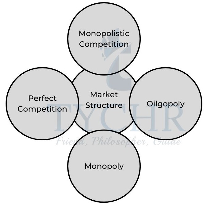
Perfect Competition
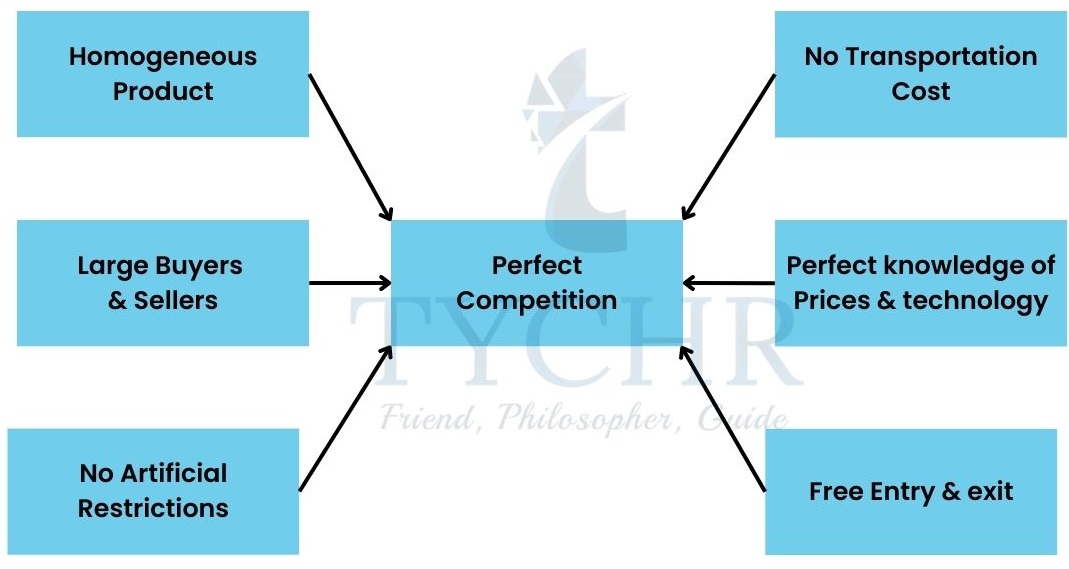
It is the market structure in which all firms in an industry are price takers and in which there is freedom of entry into and exit from industry and all firms sell homogeneous products (identical products).
Examples of perfect competition Agriculture, commodities like wheat, corn, stock exchanges, bonds market, etc.
Demand and revenue Curve
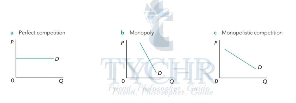
The demand curve is perfectly elastic (horizontal line). This is because the individual firm is small and can do nothing to influence the price. The firm is therefore the price taker.
Demand Curve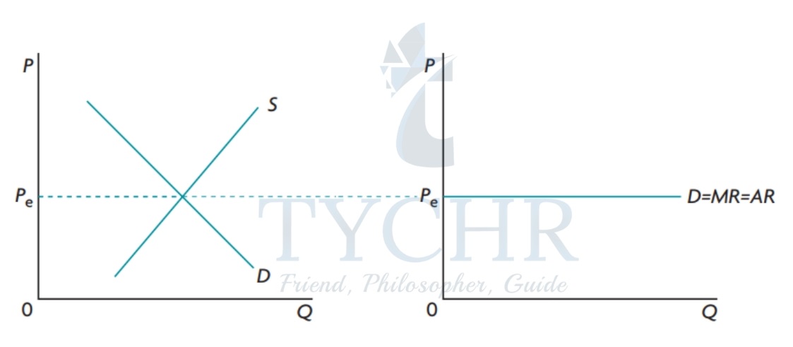
The firm’s Revenue Curve
No matter how much output the perfectly competitive firm sells, P = MR = AR and these are constant at the level of the horizontal demand curve. This follows from the fact that price is constant regardless of the level of the level of the output sold.
| Units of Output (Q) | Product Price (P) (€) | Total Revenue TR = P * Q (€) | Marginal Revenue MR = ΔTR/ΔQ | Average Revenue MR = TR / Q (€) |
| 0 | 10 | – | – | – |
| 1 | 10 | 10 | 10 | 10 |
| 2 | 10 | 20 | 10 | 10 |
| 3 | 10 | 30 | 10 | 10 |
| 4 | 10 | 40 | 10 | 10 |
| 5 | 10 | 50 | 10 | 10 |
| 6 | 10 | 60 | 10 | 10 |
| 7 | 10 | 70 | 10 | 10 |
Profit Maximisation in the short run
In the short run, the number of firms in the industry is fixed because to enter or exit, a firm must be able to vary all the inputs (which is in the long run). Since it’s a price taker, it cannot influence the selling price. It can only make a choice of how much quantity it should produce.
In the short run, at least one input is fixed (AR=MR). Based on the MR – MC approach, firms will maximize the profit when MR=MC.
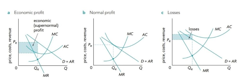
A firm can face 3 types of profit possibilities
- Economic or Supernormal profits (P>ATC).
- Break even or Normal profit (P=ATC).
- Economic loss or Subnormal profit (P<ATC).
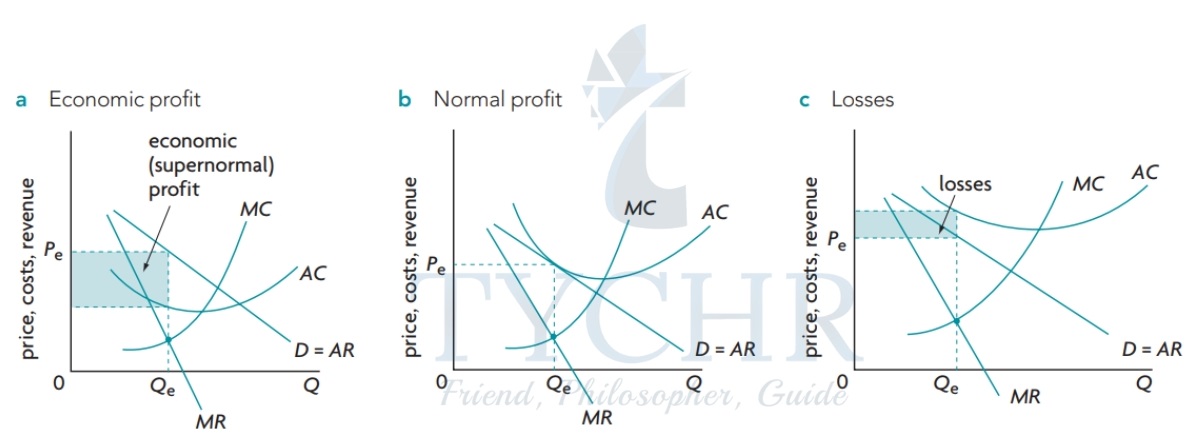
In short run
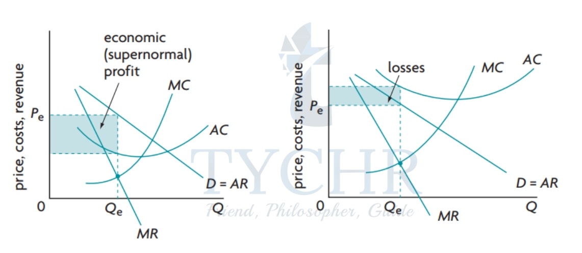
Fig 5 (a) : When P>ATC, the firm makes economic profits.
Fig 5 (b) : When P = minimum ATC, The business makes a normal profit despite making no money.This P is a break even price of the firm (break even point).
Fig 5 (c) : When ATC>P>AVC, the firm produces at a loss but it’s loss is less than fixed costs, therefore, it continues to produce.
Fig 5 (d) : When P = minimum AVC, the firm’s loss = fixed costs, this P is the firm’s short run shut – down price.
Fig 5 (e) : When P<AVC, i.e. when price falls below the shut-down price, the firm shuts down (stops producing). It’s loss will then be equal to it’s fixed costs.
Note: The portion of the perfectly competitive company’s marginal cost curve above the point of minimum AVC constitutes the short run supply curve.
Profit maximization in the long run
Firms’ economic profits and losses are eliminated in a perfectly competitive long-run equilibrium, and revenues are just enough to cover all economic costs, allowing each firm to make a normal profit.
Moving from short run to long run equilibrium
A.) Economic profit (supernormal profit) in the short run to normal profit in the long run
In the Short run
In fig 6 (b), where D and S intersect, gives the equilibrium price P, which is equal to firm’s MR and by MR – MC rule, firm produces Q ( quantity), thus earning supernormal profits = (a – b) in fig 6 (a).
In the long run
All inputs vary –> new firms enter –> supply curve shifts from S1 to S2 –> quantity increases from Q1 to Q2 –> price reduces from P1 to P2 –>economic profit => 0 => The firm earns normal profit (P= min. ATC), this is the break even price which is same for both short run and long run.
B.)In the case of Economic Loss
In the short run
As explained above, by the same MR – MC rule, in fig 6 (d), we can see, P1 = price taken by the firm and Q1 = quantity produced. Firm is earning a loss = (a – b) in fig 6 (c).
In long run
Due to losses –> firms exit –> supply curve shifts from S1 to S2 –> quantity reduces from Q1 to Q2 –> price increases from P1 to P2 –> losses = 0 –> P2 represents firm’s new MR and by MR – MC rule, firms produce output Q2 and earn normal profit (where P=minimum ATC).
The shut-down and the break-even price
- In the short run, the shut- down price is P = minimum AVC, the firm shuts down (stops producing) when price falls below minimum AVC.
- The long run shut- down price is P=minimum ATC, the firm shuts down (leaves the industry) when price falls below minimum ATC.
Allocative and Productive Efficiency
When a company produces the particular combination of goods and services that customers most frequently prefer, this is called allocation efficiency. The condition is the Cost = MC, where shopper and maker excess is greatest.
Note:
If P > MC => Under-allocation of resources.
If P < MC => Over-allocation of resources.
If P = MC => Efficient utilization of resources.
Productive (Technical) Efficiency
It occurs when production takes place at Minimum ATC, or the lowest cost possible.
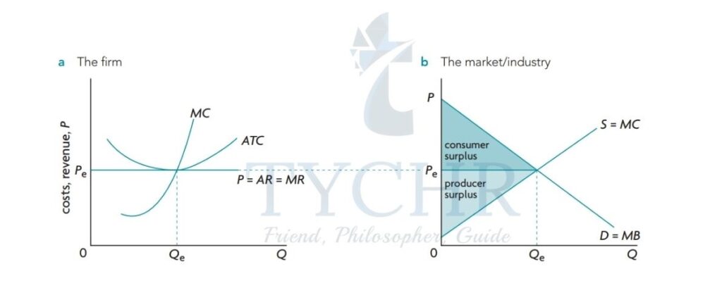
Efficiency and Perfect Competition
In the Long run: The firm achieves both Allocative efficiency (P=MC) and productive efficiency (at min. ATC).
At the level of industry, social surplus (consumer + producer surplus) is maximum and MB (demand) = MC (supply)
Short run Allocative efficiency is achieved by perfectly competitive businesses, but productive efficiency is unlikely.
Evaluating Perfect Competition
| Advantages | Disadvantages |
| Helps allocate resources to most efficient use | The conditions are very strict, there are few perfectly competitive market |
| Encourages efficiency | Insufficient profits for investment |
| Consumers benefit: consumers charged a lower price | Lack of product variety |
| Responsive to consumer wishes. | Unequal distribution of goods & income |
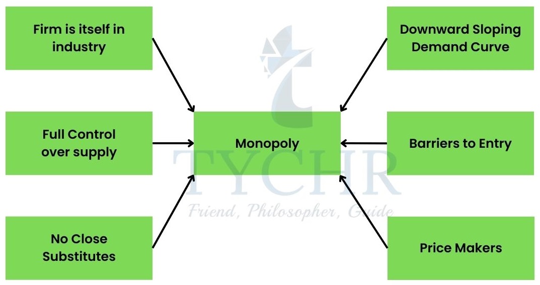
Monopoly
It is a type of market in which there is a single seller and large number of buyers selling products that have no close substitutes and have high entry and exit barriers. Eg- electricity and water provider in Sabah.
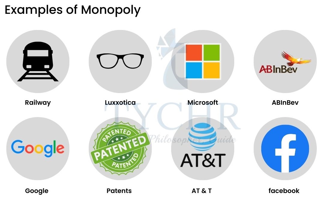
Examples of Monopoly
Barriers to entry
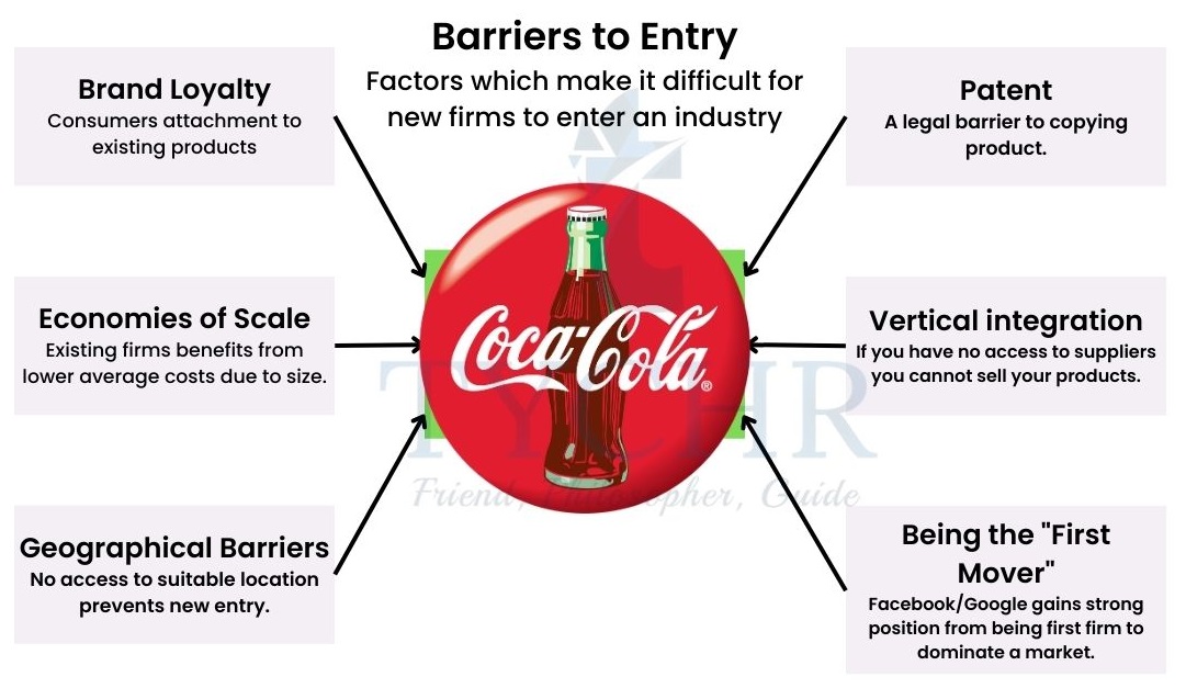
Other legal barriers are
- Patents: The rights given by a government to a firm that has developed a new product or invention, to be its sole producer for a specified period of time. Eg –new pharmaceutical products, instant cameras from Polaroid, and so on
- Licenses: It is granted by a government for a particular profession. Eg – To operate radio or television stations or to enter a particular profession. (Medicine, dentistry, etc.)
- Copyrights: A guarantee that an author has the sole right to print, publish and sell copyrighted works.
Demand and Revenue curves under Monopoly
Monopolist Demand Curve
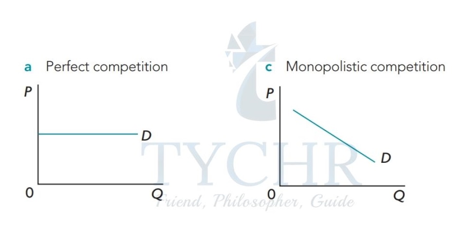
Since the pure monopolist is the entire industry, the demand curve it faces is the industry’s or market’s demand curve which is downward sloping. This is the most important difference between the monopolist and the perfectly competitive firm which faces perfectly elastic demand at the price level determined in the market.
Revenue Curve
A monopoly firm has a downward sloping demand curve which means price is changing with each level of output.
When price reduces, quantity sold is increasing
- TR increases, reaches maximum and then falls.
- MR is falling with each additional output, when MR=0, TR=maximum.
- AR= P price (since TR= PXQ and AR= TR/Q hence AR = P). AR and P represent the demand curve.
Note: MR curve lies below AR curve because here the firm must lower its price in order to sell more.
The monopolist will not produce any output in the inelastic portion of its demand curve.
Profit Maximisation by the Monopolist
The profit maximizing choice for the monopoly will be to produce at the quantity where MR=MC. At those levels of output, MR is greater than MC, and the company can increase output to make greater profits.
Note: Under monopoly high barriers to entry prevent potential competitor firms from entering a profit-making industry and the monopolist can therefore continue making supernormal (or economic) profits in the long run.
Note: The revenue maximizing monopolist produces that level of output where MR=0. Because at this point TR is maximum.
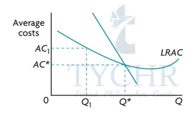
Natural Monopoly
Since MR is greater than MC at those levels of output, the business can increase output to increase profits.

Examples –
If the market demand for a product is within the range of falling LRATC, this means that a single large firm can produce for the entire market at a lower average total cost than two or more smaller firms. When this occurs, the firm is called a natural monopolist.
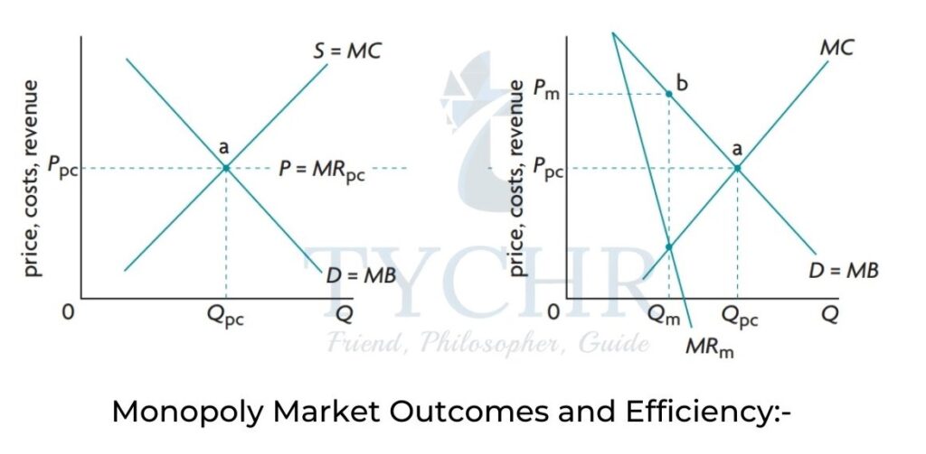
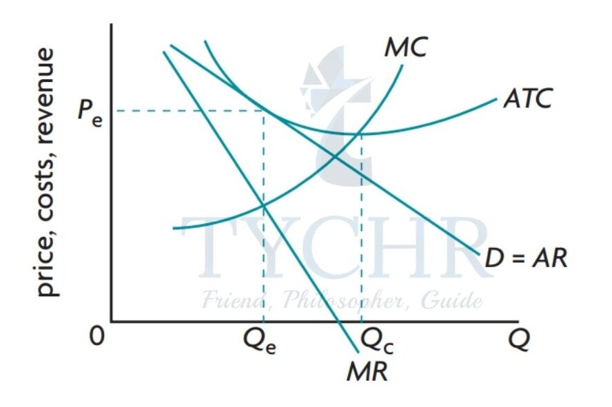
Monopoly Market Outcomes and Efficiency
In the above figure you can see, Qm < Qpc , the industry under monopoly produces a smaller quantity of output than the industry under perfect competition and since Pm>Ppc, the monopolist sells output at a higher price than the perfectly competitive market. Higher prices and lower output goes against consumer interest.
Allocative and Productive Inefficiency
Allocative Inefficiency: Lack of social surplus
The presence of dead-weight loss in monopoly indicates that there is allocative inefficiency, shown also by MB>MC at Qm, indicating too little of the good is produced. Also, the monopolist gains at the expense of consumers as a portion of consumer surplus is converted into producer surplus.
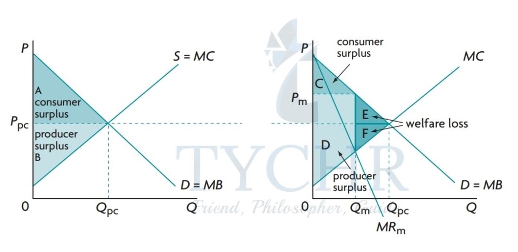
Note: In monopoly, the under-allocation of resources is indicated by P>MC at the profit maximizing level of output.
Productive Inefficiency:
Since the monopolist produces at higher than minimum average total cost (ATC), there exists productive inefficiency.
X-inefficiency (producing higher than necessary ATC)
In monopoly, the lack of competition can make the monopolist less concerned about keeping the cost low. Higher costs could arise due to poor management, lack of innovation, outdated technology, etc. This is known as X-inefficiency.
Monopolistic Competition

It is a form of imperfect competition in which a lot of producers sell products that are different from one another in some way, like by branding or quality, and are not perfect substitutes for one another. For instance, businesses like restaurants, footwear, furniture, jewelry, and clothing.
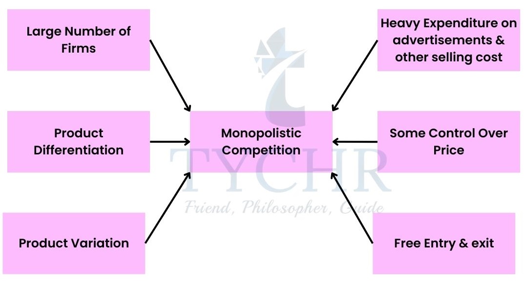
Note: Product differentiation means one product differs from another. There could be
Physical differences (size, shape, taste, packaging) eg- Colgate differs from Pepsodent.
Quality differences
Location
Services (like after sales service, demonstrations)
Product image (celebrity advertising or endorsements)
Demand and Revenue Curve
It is the same as monopoly with higher price elasticity. Every firm has a mini monopoly in a good it produces eg- Nike has a monopoly in Nike shoes, Adidas has a monopoly in Adidas shoes. If the price of Adidas shoes rises, not all buyers (who are brand loyal) will shift to another brand, while some might shift to Nike.
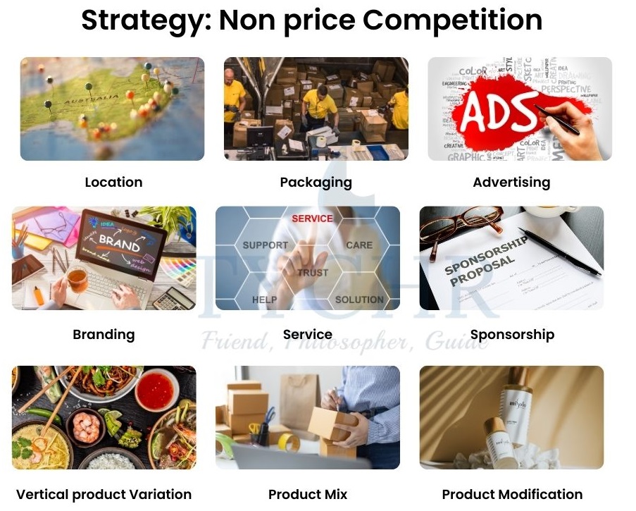
Price and Non-price Competition
Profit Maximisation
Short run
The demand curve is more elastic and flatter in monopolistic competition than in monopoly. In the short run, firm can make either supernormal profits or losses.
Long run
Long-term, profitable industries draw new competitors. Some businesses shut down and leave industries that make losses. In the long run, the process by which businesses enter and exit ensures that there is no economic profit or loss and that all businesses make a normal profit.
Allocative and Productive Inefficiency
In monopolistic competition, neither distributive nor productive efficiency can achieve long-term equilibrium for the company.
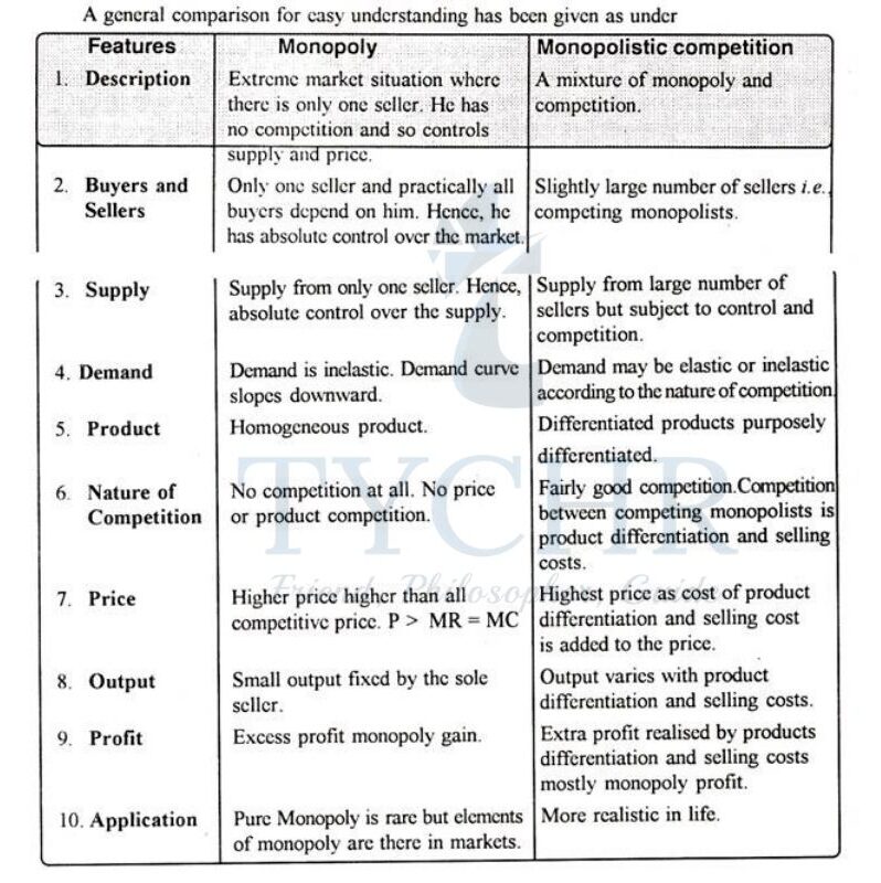
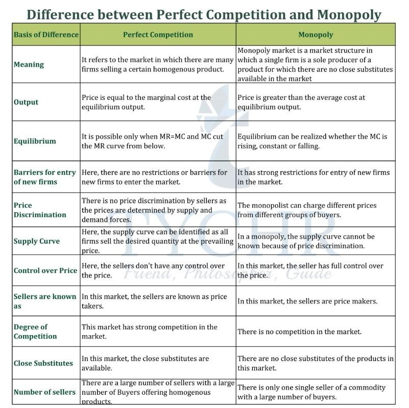
Comparisons
Monopolistic and perfect competition
Monopolistic Competition and Monopoly
Oligopoly
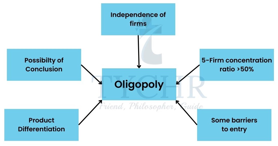
Note:
Example of differentiated products – aircrafts, cars, etc. Example of homogenous products – oils, steel, aluminum, etc.
Strategic Behaviour and Conflicting Incentives
Strategic Behaviour
It is based on plans of action that consider the possible actions of competitors. like chess or a card game.
Conflicting Incentives
The firm faces 2 conflicting incentives
Incentive to collude: Collusion refers to an agreement between the firms to limit competition between them.
Incentive to compete: Each firm faces an incentive to compete with its rival so as to capture the rival’s market share.
Explanation of Oligopolistic behavior by use of Game Theory
Game theory It is a mathematical technique analyzing the behavior of decision makers who are dependent on each other and who use strategic behavior as they try to anticipate the behavior of their rivals.
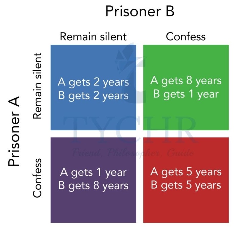
Nash equilibrium and Prisoner’s Dilemma Occasionally, Nash equilibrium demonstrates a conflict between individual self-interest and the collective firm’s interest. Prisoner’s Dilemma is the name given to this dispute. Even though co-operation could improve the company’s financial situation, every company that tries to improve its own situation ends up hurting both itself and its rival.
Example
The Concentration Ratio
It tells you how much of an industry’s output is produced by the biggest companies. A concentration is determined for any number of businesses, but there is no set number. For instance, a ratio of four firms that is 75% indicates that the industry’s top four firms generate 75% of all sales.
Criticism
- Provides no indication of the importance of firms in the global market.
- It neglects competition from other industries.
Collusive Oligopoly
If the firms cooperate with each other in determining price or output or both, it is called collusive oligopoly or cooperative oligopoly. In other words, the firms in a collusive oligopoly combines to avoid the competition among themselves regarding the price and output of the industry. For example, OPEC(Organization for petroleum exporting countries) serves the example for collusive oligopolies.

Open / Formal Cartels
It is defined as a group of firms, that get together to make output and price decisions. They form cartels to increase market power, control level of output and price.
Tacit/ Informal collusion : Price Leadership:
Without a formal agreement, it refers to co-operation that is implicit or understood between the cooperating businesses.
Non Collusive Oligopoly: The Kinked Demand Curve
The firms do not form groups, they work independently.
Non-price Competition in Oligopoly (no change in price)
Advertisement and R and D
Product diversification (new product or product line)
Product differentiation
Price Discrimination
Refers to the selling or charging different prices by a firm to different buyers for a similar product. The difference in prices by a firm to different buyers for similar product is not associated with costs. E.g. Firm charging lower rate to children, does not mean that firm would reduce their profit. Because price discrimination is potentially profitable, businesses have found many ways to do it. E.g. Price charged for movie ticket is different between adults, children and senior citizens.
Three conditions for price discrimination
Three Necessary Conditions for Price Discrimination
1) Some degree of market power
2) Seller must have some means of approximating what different buyers are willing (the maximum) to pay for each unit of output
3.) Seller must be able to prevent resale (or arbitrage) of the product
Note: Different price elasticity of demand Consumers must have different PEDs for the good. This is because consumers with a relatively low PED will be willing to pay a higher price for a good.