By the end of this chapter you should be familiar with:
- Concept of a limit
- Derivatives of standard functions
- Chain rule, product rule and quotient rule
- Tangents and normal
- Increasing and decreasing functions
- The second derivative
- Optimization
- Related rates
LIMITS AND DERIVATIVES
LIMITS
Suppose we have a function f(x). The value, a function attains, as the variable x approaches a particular value say a, i.e., x → a is called its limit. Here, ‘a’ is some pre-assigned value. It is denoted as limx→af(x) = 1
- The expected value of the function shown by the points to the left of a point ‘a’ is the left-hand limit of the function at that point. It is denoted as limx→a− f(x).
- The points to the right of a point ‘a’ which shows the value of the function is the right-hand limit of the function at that point. It is denoted as limx→a+ f(x).
Limits of functions at a point are the common and coincidence value of the left and right-hand limits.
The value of a limit of a function f(x) at a point a i.e., f(a) may vary from the value of f(x) at ‘a’.
If the function after applying limits is in the 0/0 or ∞/∞ form then you differentiate the numerator and the denominator until it’s not in 0/0 or ∞/∞ form.
Example: Find the limit of limx→2 [x3 + 2x2 + 4x – 2]
Solution: limx→2 [x3 + 2x2 + 4x – 2] = limx→2 x3 + 2 limx→2 x2 + 4 limx→2 x – limx→2 2
= 23 + 2×22 + 4×2 − 2 = 22
DERIVATIVE
Assume a function f(x) within its domain. Let us say, this function involves the calculation of the rate of change of velocity or as we know it the acceleration of a vehicle as it moves from one point to the other.
Now obviously the rate of change of velocity is instantaneous as the function is dependent on both the speed as well as the direction of the vehicle. If we are to find the instantaneous acceleration of the vehicle we will need the limits of the function at that instant.
A function denoting the rate of change of another function is called as a derivative of that function. In other words, a derivative is used to define the rate of change of a function.
The derivative of a function f(x) at any point ‘a’ in its domain is given by: limh->0 [f(a+h) – f(a)]/h
If the derivative exists. It is denoted by f'(a) and f'(a) changes as the value of x changes in its domain
Solution: The derivative of a function f(x) at a point is given by: f ‘(x) = lim h -> 0 [f(x+h) – f(x)]/h
So, f’(x=1) = lim h -> 0 [(2(1+h)2+3(1+h)-5)-(2+3-5)]/h = lim h -> 0 [(2h2-h)]/h = lim h->0 {2h – 1} = -1
Before we get into the next topic lets look at some rules.
CHAIN RULE
The chain rule states that the derivative of f(g(x)) is f'(g(x))⋅g'(x). In other words, it helps us differentiate composite functions. Basically: d[ f(g(x)) ]/dx = f’(g(x)) × g’(x)
Here is a list of derivates of common function so you don’t have to keep using the formula again and again:

Example: Let f(x)=ex and g(x)=4x. Use the chain rule to calculate h′(x), where h(x)=f(g(x)).
Solution: The derivate of a exponential function with base e is just the function itself,
So, f′(x)=ex and the derivative of g is g′(x)=4.
According to the chain rule,
d[ f(g(x))]/dx = f’(g(x)) × g’(x)
h′(x) = f′(g(x)) × g′(x)
= f′(4x) × 4 = 4e4x
PRODUCT AND QUOTIENT RULE
If the two functions f(x) and g(x) are differentiable then the product is differentiable and
(f(x)g(x))′ = f′(x)g(x) + f(x)g′(x) [PRODUCT RULE]
If the two functions f(x)f(x) and g(x)g(x) are differentiable (i.e. the derivative exist) then the quotient is differentiable and,
(f(x)/g(x))′ = (f′(x)g(x) – f(x)g′(x))/𝑔(𝑥)2
Example: Find the differentiation of the following functions:
- f(x) = (6x3 − x)(10 − 20x)
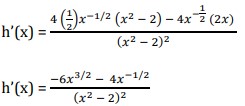
- h(x) = 4√𝑥/(𝑥2−2)
Solution:
- Using the product rule,
f′(x) = (18x2 − 1)(10 − 20x) + (6x3 − x)(−20)
= −480x3 + 180x2 + 40x – 10 - Using the quotient rule,
TANGENTS AND NORMALS
A tangent to a curve is a line that touches the curve at one point and has the same slope as the curve at that point.
A normal to a curve is a line perpendicular to a tangent to the curve.
Note 1: We can find the slope of a tangent at any point (x, y) using dy/dx.
Note 2: To find the equation of a normal, recall the condition for two lines with slopes m1 and m2 to be perpendicular is m1 × m2 = −1.
Example:
- Find the gradient of the tangent and the normal to the curve y = x3− 2x2 + 5 at the point (2,5).
- Find the equation of the tangent and the normal.
- Sketch the graph.
Solution:
- dy/dx = 3x2 − 4x
The slope of the tangent is m1 = [dy/dx]x=2
= 12 – 8 = 4
The slope of normal m2 = -1/m1 [Using m1m2 = -1]
m2 = -1/4 - Using the formula y – y1 = m(x – x1)
For tangent, substituting m = 4 we get
y – 5 = 4(x – 2)
4x – y – 3 =0
For normal, substituting m = -1/4 we get
y – 5 = (-1/4)(x – 2)
x + 4y – 22 = 0 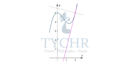

MINIMA, MAXIMA AND POINTS OF INFLECTION
INCREASING AND DECREASING FUNCTIONS
A function is increasing on an interval if for any x1 and x2 in the interval then,
x1 < x2 implies f(x1) < f(x2)
A function is decreasing on an interval if for any x1 and x2 in the interval then,
x1 < x2 implies f(x1) > f(x2)
Let f be a differentiable function on the interval (a, b) then [this is also known as the first derivative test]
- If f ‘(x) < 0 for x in (a, b), then f is decreasing there and the point is known as local minimum.
- If f ‘(x) > 0 for x in (a, b), then f is increasing there and the point is known as local maximum.
- If f ‘(x) = 0 for x in (a, b), then f is constant.
We say that x = c is a critical point of a function f(x) if f(c) exists and either of the following are true:
f’(c) = 0 or f’(c) doesn’t exist.
An Inflection Point is where a curve changes from Concave upward to Concave downward or vice versa.
Example: Determine the values of x where the function f(x) = 2x3 + 3x2 – 12x + 7
Solution: We first take the derivative f ‘(x) = 6x2 + 6x – 12
To determine where the derivative is positive and where it is negative, find the roots.
Factor to get: 6(x2 + x – 2) = 6(x – 1)(x + 2)
Hence the change in sign can occur when x = 1 and x = -2 which are also known as the critical points.
x | f ‘(x) |
-3 | 24 |
0 | -12 |
2 | 24 |
Now create some test values
The derivative is positive outside of [-2,1] and is negative inside of [-2,1].
We can conclude that f(x) is increasing outside of [-2,1] and decreasing inside of [-2,1].
The graph is shown below.
To find absolute maximum or minimum we need to find local extrema and then compare then to see which one is the greatest or least value for the entire domain of f(x). The function may have more than one local extremum.
Example: Find the absolute extrema of h(x) = 2x3 + 3x2 – 12 over the interval -3 ≤ x ≤ 3
Solution: h′(x) = 6(x + 2)(x − 1), so our critical points are x = -2 and x=1. They divide the closed interval -3 ≤ x ≤ 3 into three parts:
So now lets make a table.
Interval | x-value | h’(x) | Verdict |
-3 < x < -2 | x = -5/2 | h’(-5/2) = 21/2 > 0 | increasing |
-2 < x < 1 | x = 0 | h’(0) = -12 < 0 | decreasing |
1 < x < 3 | x = 2 | h’(2) = 24 > 0 | increasing |
Now we look at the critical points and the endpoints of the interval:
x | h(x) | Before | After | Verdict |
-3 | 9 | none | increasing | Minimum |
-2 | 20 | increasing | decreasing | Maximum |
1 | -7 | decreasing | increasing | Minimum |
3 | 45 | increasing | none | Maximum |
On the closed interval −3≤ x ≤3, the points (-3, 9) and (1, -7) are relative minima and the points (-2, 20) and (3, 45) are relative maxima.
(1, -7) is the lowest relative minimum, so it’s the absolute minimum point and (3,45 is the largest relative maximum, so it’s the absolute maximum point.
Notice that the absolute minimum value is obtained within the interval and the absolute maximum value is obtained on an endpoint.
SECOND DERIVATIVE TEST
Suppose f(x) is a function of x that is twice differentiable at a stationary point x0.
- If f’’(x0) > 0, then f has a local minimum at x0.
- If f’’(x0) < 0, then f has a local maximum at x0.
The extremum test gives slightly more general conditions under which a function with f’’(x0) = 0 is a maximum or minimum.
If f(x, y) is a two – dimensional function that has a local extremum at a point (x0, y0) and has continuous partial derivatives at this point, then fx(x0, y0) and fy(x0, y0). The second partial derivatives test classifies the point as a local maximum or local minimum.
We define the second derivative test discriminant as
D ≡ fxx fyy – fxy fyx
D = fxx fyy – (fxy)2
Then
- If D > 0 and fxx(x0, y0) > 0, the point is a local minimum.
- If D > 0and fxx(x0, y0) < 0, the point is a local maximum.
- If D < 0, the point is a saddle point.
- If D = 0, higher order tests must be used.
Example: Consider f(x) = sinx + cosx
f′(x) = cosx – sinx
f′′(x) = −sinx −cosx
Since f′′(π/4) = -1/√2 – 1/√2 = – √2< 0 there is a local maximum at π/4.
Since f′′(5π/4) = 1/√2 + 1/√2= √2> 0 there is a local minimum at 5π/4.
To summarize,
OPTIMISATION
In optimization problems we are looking for the largest value or the smallest value that a function can take. Here we will be looking for the largest or smallest value of a function subject to some kind of constraint. The constraint will be some condition (that can usually be described by some equation) that must absolutely, positively be true no matter what our solution is.
Example: We want to construct a box whose base length is 3 times the base width. The material used to build the top and bottom cost $10/ft2 and the material used to build the sides cost $6/ft2. If the box must have a volume of 50ft3 determine the dimensions that will minimize the cost to build the box.
Solution: 
The two functions we’ll be working with here this time are,
Minimize: C = 10(2lw) + 6(2wh + 2lh) = 60w2 + 48wh
Constraint: 50 = lwh = 3w2h
We will solve the constraint for one of the variables and plug this into the cost. It will definitely be easier to solve the constraint for h so let’s do that.
h = 50/3w2
Plugging this into the cost gives,
C(w) = 60w2 + 48w(50/3w2) = 60w2 + 800/w
Now, let’s get the first and second derivatives,
C′(w) = 120w − 800w-2
C′′(w) = 120 + 1600w-3
Now we need the critical point for the cost function. First, notice that w=0 is not a critical point. Clearly the derivative does not exist at w=0 but then neither does the function and remember that values of w will only be critical points if the function also exists at that point.
120w3 – 800 = 0
w = 1.8821 which is the critical point and gives absolute minimum cost.
l = 3w = 3(1.8821) = 5.6463
h = 50/3w2 = 50/3(1.8821)2 = 4.7050
C(1.8821) = $637.60
RELATED RATES
Related rates look at the effect that a change in a particular rate has on another rate.
Here are the steps in doing a related rates problem:
- Decide what the two variables are.
- Find an equation relating them.
- Take d/dtof both sides.
- Plug in all known values at the instant in question.
- Solve for the unknown rate.
Example: You are inflating a spherical balloon at the rate of 7 cm3/sec. How fast is its radius increasing when the radius is 4 cm?
Solution: Here the variables are the radius r and the volume V.
We know dV/dt, and we want dr/dt. The two variables are related by means of the equation:
V = 4πr3/3.
Taking the derivative of both sides gives:
dV/dt = 4πr2r’ 7 = 4π (4)2 r’ r’ = 7/64π cm/sec = 0.0348 cm/sec
