By the end of this chapter you should be familiar with:

• Simple, weighted and directed graphs
• Minimum spanning tree
• Adjacency and transition matrices
• Eulerian circuits and trails
• Hamiltonian paths and cycles
• Tables of least distances
• Classical and practical travelling salesman problems

A graph is defined as set of vertices and a set of edges. A vertex represents an object. An edge joins two vertices.

A graph with no loops and no parallel edges is called a simple graph.

• The maximum number of edges possible in a single graph with ‘n’ vertices is ⁿC₂.
• The number of simple graphs possible with ‘n’ vertices =(2)^(nC2)

The graph that shows values like cost, time, distance, etc., are known as weighted graphs.
In a directed graph, each edge has a direction.

A graph G is said to be connected if there exists a path between every pair of vertices. There should be at least one edge for every vertex in the graph. So that we can say that it is connected to some other vertex at the other side of the edge.

The degree (or order) of a vertex in a graph is the number of edges with that vertex as an end point.
A vertex whose degree is an even number is said to have an even degree or even vertex.

The in-degree of a vertex in a directed graph is the number of edges with that vertex as an end point. The out-degree of a vertex in a directed graph is the number of edges with that vertex as a starting point.

A graph having no edges is called a Null Graph.

A simple graph with ‘n’ mutual vertices is called a complete graph and it is denoted by ‘K_n’. In the graph, a vertex should have edges with all other vertices, then it called a complete graph.

In other words, if a vertex is connected to all other vertices in a graph, then it is called a complete graph.

A simple graph G = (V, E) with vertex partition V = {V₁, V₂} is called a bipartite graph if every edge of E joins a vertex in V₁ to a vertex in V₂.

In general, a Bipartite graph has two sets of vertices, let us say, V₁ and V₂, and if an edge is drawn, it should connect any vertex in set V₁ to any vertex in set V₂.

A bipartite graph ‘G’, G = (V, E) with partition V = {V₁, V₂} is said to be a complete bipartite graph if every vertex in V₁ is connected to every vertex of V₂.

In general, a complete bipartite graph connects each vertex from set V₁ to each vertex from set V₂.

Example: The following graph is a complete bipartite graph because it has edges connecting each vertex from set V₁ to each vertex from set V₂.

If |V₁| = m and |V₂| = n, then the complete bipartite graph is denoted by K_{m, n}.

• K_m,n has (m+n) vertices and (mn) edges.
• K_m,n is a regular graph if m=n.

In general, a complete bipartite graph is not a complete graph.
K_m,n is a complete graph if m=n=1.
The maximum number of edges in a bipartite graph with n vertices is n²/4
If n = 10, k5, 5 = n²/4 = 100/4 = 25
Similarly,
K6, 4 = 24
K7, 3 = 21
K8, 2 = 16
K9, 1 = 9

If n = 9, k5, 4 = n²/4 = 81/4 = 20
Similarly,
K6, 3 = 18
K7, 2 = 14
K8, 1 = 8

‘G’ is a bipartite graph if ‘G’ has no cycles of odd length. A special case of bipartite graph is a star graph.

GRAPH REPRESENTATION

ADJACENCY MATRICES

For a graph with |V| vertices, an adjacency matrix is a ∣V∣×∣V∣ matrix of 0s and 1s, where the entry in row i and column j is 1 if and only if the edge (i, j) is in the graph. If you want to indicate an edge weight, put it in the row i, column j entry, and reserve a special value (perhaps null) to indicate an absent edge. Here’s the adjacency matrix for the social network graph:

Example:

INCIDENCE MATRICES

Let G be a graph with n vertices, m edges and without self-loops. The incidence matrix A of G is an n × m matrix A = [a_ij] whose n rows correspond to the n vertices and the m columns correspond to m edges such that:
a_i,j = 1 if jth edge m_j is incident on the i^th vertex else it’s 0.

Example:

TRANSITION MATRICES

The transition matrix A associated to a directed graph is defined as follows. If there is an edge from i to j and the outdegree of vertex i is di, then on column i and row j we put 1/d_i. Otherwise we mark column i, row j with zero. Notice that we first look at the column, then at the row. We usually write 1/d_i on the edge going from vertex i to an adjacent vertex j, thus obtaining a weighted graph.

Example: Then the transition matrix associated to it is:

In general, a matrix is called primitive if there is a positive integer k such that A^k is a positive matrix. A graph is called connected if for any two different nodes i and j there is a directed path either from i to j or from j to i. On the other hand, a graph is called strongly connected if starting at any node i we can reach any other different node j by walking on its edges.

The direction of movement in a transition matrix is opposite to that of an adjacency matrix.

THE MINIMUM SPANING TREE

Given an undirected and connected graph G = (V, E), a spanning tree of the graph G is a tree that spans G (that is, it includes every vertex of G) and is a subgraph of G (every edge in the tree belongs to G)

A cycle is walk that begins and ends at the same vertex.

The cost of the spanning tree is the sum of the weights of all the edges in the tree. There can be many spanning trees. Minimum spanning tree is the spanning tree where the cost is minimum among all the spanning trees. There also can be many minimum spanning trees.

Minimum spanning tree has direct application in the design of networks. It is used in algorithms approximating the travelling salesman problem, multi-terminal minimum cut problem and minimum-cost weighted perfect matching.

KRUSHKAL’S ALGORITHM

Kruskal’s Algorithm builds the spanning tree by adding edges one by one into a growing spanning tree. Kruskal’s algorithm follows greedy approach as in each iteration it finds an edge which has least weight and add it to the growing spanning tree.

Algorithm Steps:

• Sort the graph edges with respect to their weights.
• Start adding edges to the MST from the edge with the smallest weight until the edge of the largest weight.
• Only add edges which doesn’t form a cycle, edges which connect only disconnected components.

PRIM’S ALGORITHM

Prim’s Algorithm also use Greedy approach to find the minimum spanning tree. In Prim’s Algorithm we grow the spanning tree from a starting position. Unlike an edge in Kruskal’s, we add vertex to the growing spanning tree in Prim’s.

Algorithm Steps:

• Maintain two disjoint sets of vertices. One containing vertices that are in the growing spanning tree and other that are not in the growing spanning tree.
• Select the cheapest vertex that is connected to the growing spanning tree and is not in the growing spanning tree and add it into the growing spanning tree. This can be done using Priority Queues. Insert the vertices, that are connected to growing spanning tree, into the Priority Queue.
• Check for cycles. To do that, mark the nodes which have been already selected and insert only those nodes in the Priority Queue that are not marked.

In Kruskal’s algorithm, at each iteration we will select the edge with the lowest weight. So, we will start with the lowest weighted edge first i.e., the edges with weight 1. After that we will select the second lowest weighted edge i.e., edge with weight 2. Notice these two edges are totally disjoint. Now, the next edge will be the third lowest weighted edge i.e., edge with weight 3, which connects the two disjoint pieces of the graph. Now, we are not allowed to pick the edge with weight 4, that will create a cycle and we can’t have any cycles. So, we will select the fifth lowest weighted edge i.e., edge with weight 5. Now the other two edges will create cycles so we will ignore them. In the end, we end up with a minimum spanning tree with total cost 11 (1 + 2 + 3 + 5).

In Prim’s Algorithm, we will start with an arbitrary node (it doesn’t matter which one) and mark it. In each iteration we will mark a new vertex that is adjacent to the one that we have already marked. As a greedy algorithm, Prim’s algorithm will select the cheapest edge and mark the vertex. So, we will simply choose the edge with weight 1. In the next iteration we have three options, edges with weight 2, 3 and 4. So, we will select the edge with weight 2 and mark the vertex. Now again we have three options, edges with weight 3, 4 and 5. But we can’t choose edge with weight 3 as it is creating a cycle. So, we will select the edge with weight 4 and we end up with the minimum spanning tree of total cost 7 (1 + 2 +4).

THE CHINESE POSTMAN PROBLEM

A connected graph G is Eulerian if there exists a closed trail containing every edge of G. Such a trail is an Eulerian trail. Note that this definition requires each edge to be traversed once and once only, A non-Eulerian graph G is semi-Eulerian if there exists a trail containing every edge of G.

These are Eulerian, semi-Eulerian and non-Eulerian graphs respectively.

A trail is walk that repeats no edges. A circuit is a trail that starts and finishes at the same vertex.

The problem is how to find a shortest closed walk of the graph in which each edge is traversed at least once, rather than exactly once. In graph theory, an Euler cycle in a connected, weighted graph is called the Chinese Postman problem.

To find a minimum Chinese postman route we must walk along each edge at least once and in addition we must also walk along the least pairings of odd vertices on one extra occasion. An algorithm for finding an optimal Chinese postman route is:

1. List all odd vertices.
2. List all possible pairings of odd vertices.
3. For each pairing find the edges that connect the vertices with the minimum weight.
4. Find the pairings such that the sum of the weights is minimised.
5. On the original graph add the edges that have been found in Step 4.
6. The length of an optimal Chinese postman route is the sum of all the edges added to the total found in Step 4.
7. A route corresponding to this minimum weight can then be easily found.

Example:

1. The odd vertices are A and H.
2. There is only one way of pairing these odd vertices, namely AH.
3. The shortest way of joining A to H is using the path AB, BF, FH, a total length of 160.
4. Draw these edges onto the original network.
   
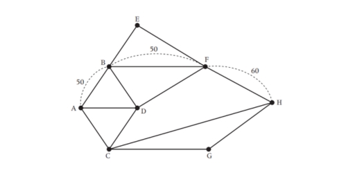
5. The length of the optimal Chinese postman route is the sum of all the edges in the original network, which is 840 m, plus the answer found in Step 4, which is 160 m. Hence the length of the optimal Chinese postman route is 1000 m.
6. One possible route corresponding to this length is ADCGHCABDFBEFHFBA, but many other possible routes of the same minimum length can be found.

TRAVELLING SALESMAN PROBLEM

A path is a walk which does not pass through any vertex more than once. A cycle is a walk that begins and ends at the same vertex, but otherwise does not pass through any vertex more than once.

A Hamiltonian path or cycle is a path or cycle which passes through all the vertices in a graph.

The classical travelling salesman problem (TSP) is to find the Hamiltonian cycle of least weight in a complete weighted graph.

The practical TSP is to find the walk of least weight that passes through each vertex of a graph. In this case the graph need not be complete.

Suppose a salesman wants to visit a certain number of cities allotted to him. He knows the distance of the journey between every pair of cities. His problem is to select a route the starts from his home city, passes through each city exactly once and return to his home city the shortest possible distance. This problem is closely related to finding a Hamiltonian circuit of minimum length. If we represent the cities by vertices and road connecting two cities edges we get a weighted graph where, with every edge e_i a number w_i(weight) is associated.

A physical interpretation of the above abstract is: consider a graph G as a map of n cities where w (i, j) is the distance between cities i and j. A salesman wants to have the tour of the cities which starts and ends at the same city includes visiting each of the remaining a cities once and only once.

In the graph, if we have n vertices (cities), then there is (n-1)! Edges (routes) and the total number of Hamiltonian circuits in a complete graph of n vertices will be (n – 1)!/2

FINDING AN UPPER BOUND

An upper bound can be found using the nearest neighbour algorithm:

Step1: Select an arbitrary vertex and find the vertex that is nearest to this starting vertex to form an initial path of one edge.

Step2: Let v denote the latest vertex that was added to the path. Now, among the result of the vertices that are not in the path, select the closest one to v and add the path, the edge-connecting v and this vertex. Repeat this step until all the vertices of graph G are included in the path.

Step3: Join starting vertex and the last vertex added by an edge and form the circuit.

This will always produce a valid Hamiltonian cycle, and therefore must be at least as long as the minimum cycle. Hence, it is an upper bound. By choosing different starting vertices, a number of different upper bounds can be found.

The best upper bound is the upper bound with the smallest value.

FINDING A LOWER BOUND

Lower bounds can be found by using spanning trees. Since removal of one edge from any Hamilton cycle yields a spanning tree, we see that solution to TSP > minimum length of a spanning tree (MST).

Consider any vertex v in the graph G. Any Hamilton cycle in G has to consist of two edges from v, say vu and vw, and a path from u to w in the graph G \ {v} obtained from G by removing v and its incident edges. Since this path is a spanning tree of G \ {v}, we have Solution to TSP ≥ (sum of lengths of two shortest edges from v) + (MST of G \ {v}).

An alternative is to use the deleted vertex algorithm.

The method for finding a lower bound:

1. Delete a vertex and find the minimum spanning tree for what remains.
2. Reconnect the vertex you deleted using the two smallest arcs.
3. Repeat this process for all vertices and select the highest as the best lower bound.

Example 1: Use the nearest-neighbour method to solve the following travelling salesman problem, for the graph shown in fig starting at vertex v₁.

Solution: We have to start with vertex v₁. By using the nearest neighbour method, vertex by vertex construction of the tour or Hamiltonian circuit is shown in fig:

The total distance of this route is 18.

Example 2: Find a lower bound by deleting vertex A from the graph.

Solution: With the vertex A deleted, the minimum spanning tree is:

This has weight = 25.

The two deleted edges of least weight have weights of 4 and 5.

Lower bound = 25 + 5 + 4 = 34