Production in the short run: Law of diminishing returns
Short Run | Long Run |
It is a time period during which at least one input is fixed and cannot be changed by the firm. Eg Land, building | It is a time period when all inputs can be changed. Eg- Firm can buy buildings, machinery,etc. |
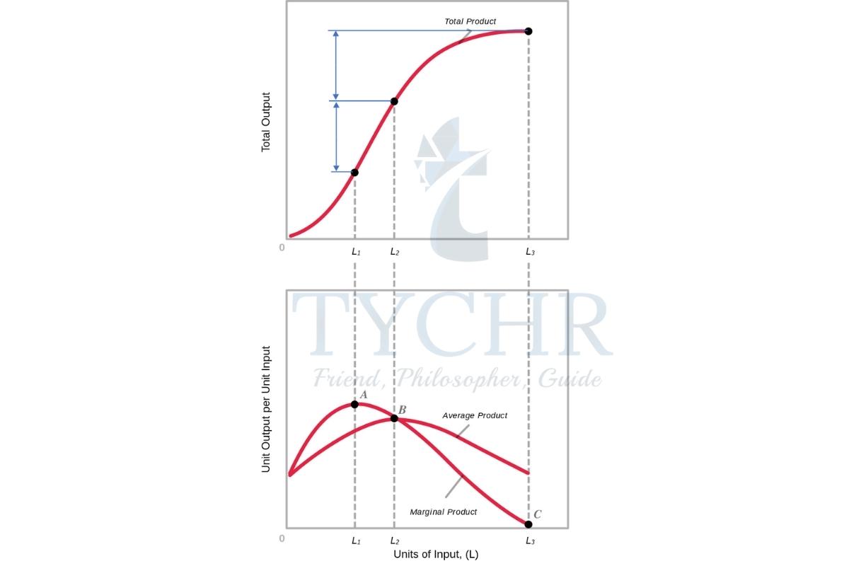
Total product, marginal product and average product
Total Product (TP)= total quantity of output produced by a firm.
Marginal Product (MP) = Extra or additional output resulting from one additional unit of the variable input. Eg- labour.
MP = change in TP/change in units of labour.
Average Product (AP) = It is the total quantity of output per unit of variable input or labour. It tells us how much output each unit of labour produces on average
.AP = TP/units of labour.
Increasing MP When labour units are between 0 to 4, with addition to TP, MP also increases and is maximum at 5 units.
Decreasing MP Between 4 and 9 labour units. Here, in addition to TP made by successive units of labour becomes smaller and smaller.
Negative MP Between 8 and 9 units of labour. TP is maximum at 9 units. Here MP=0. After 9 units of labour, TP falls and MP is negative.
Relation between AP and MP
- When MP>AP or lies above AP – AP is increasing.
- When MP<AP or lies below AP – AP is decreasing.
- When MP=AP – AP is maximum.
Law of Diminishing Returns
According to the above law (also known as law of diminishing marginal product), as more and more units of a variable input (such as labour) are added to one or more fixed inputs (such as land), the MP at first increases, but there comes a point where it begins to decrease. This relationship assumes that the fixed inputs remain fixed and technology of production is also fixed.
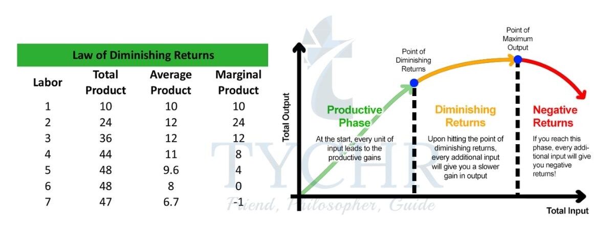
Initially with the increase in labour, TP is increasing at an increasing rate, MP also increases till 2 units of labour.
After that TP increases at a diminishing rate and is maximum at 5 and 6 units of labour, MP starts falling and becomes 0 at 6th unit.
After that TP starts falling, MP becomes negative due to additional units of labour.
Introduction to Costs of Production
Cost of Production The expenses incurred on all the factor services used for the production of a commodity are known as cost of production. Eg – wages to labour, raw material costs, salaries, electricity charges, etc.
Note: In economics, because of the condition of scarcity, economic costs, which include all costs of production, are opportunity costs of all resources used in production.
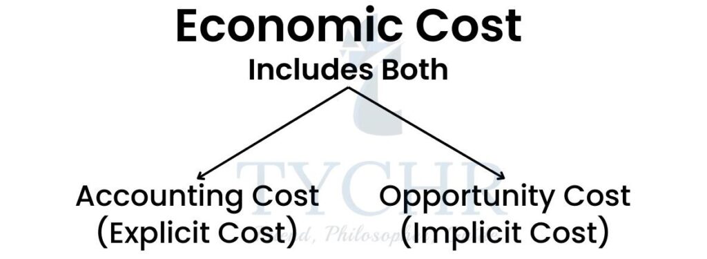
Implicit and Explicit Cost
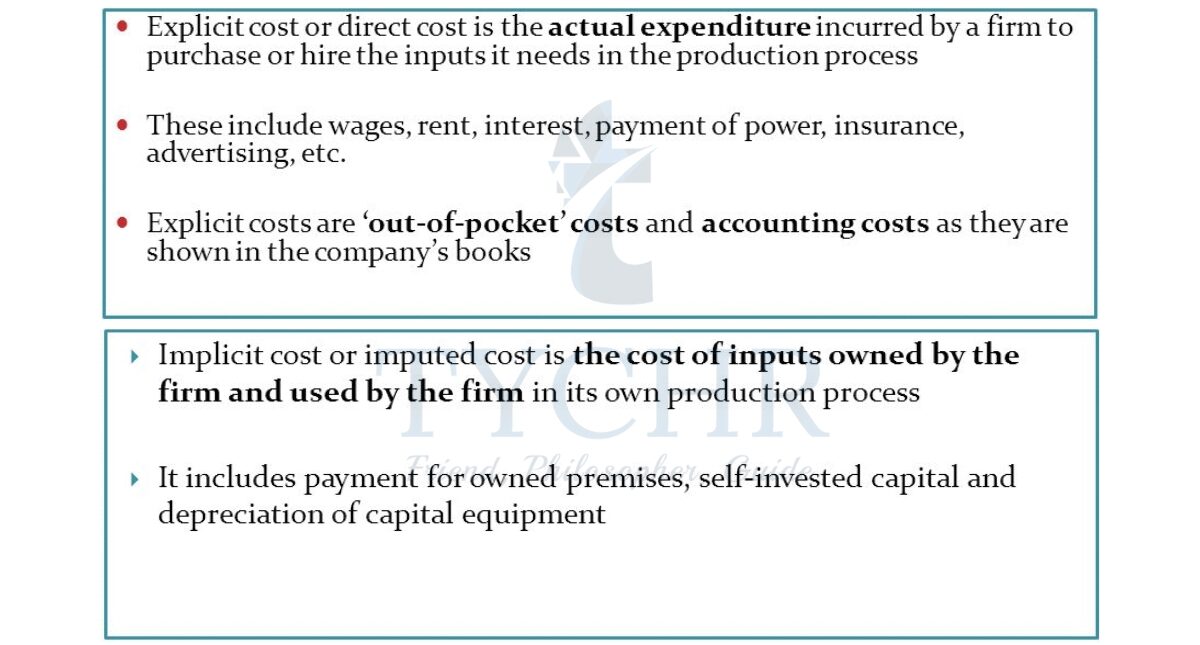
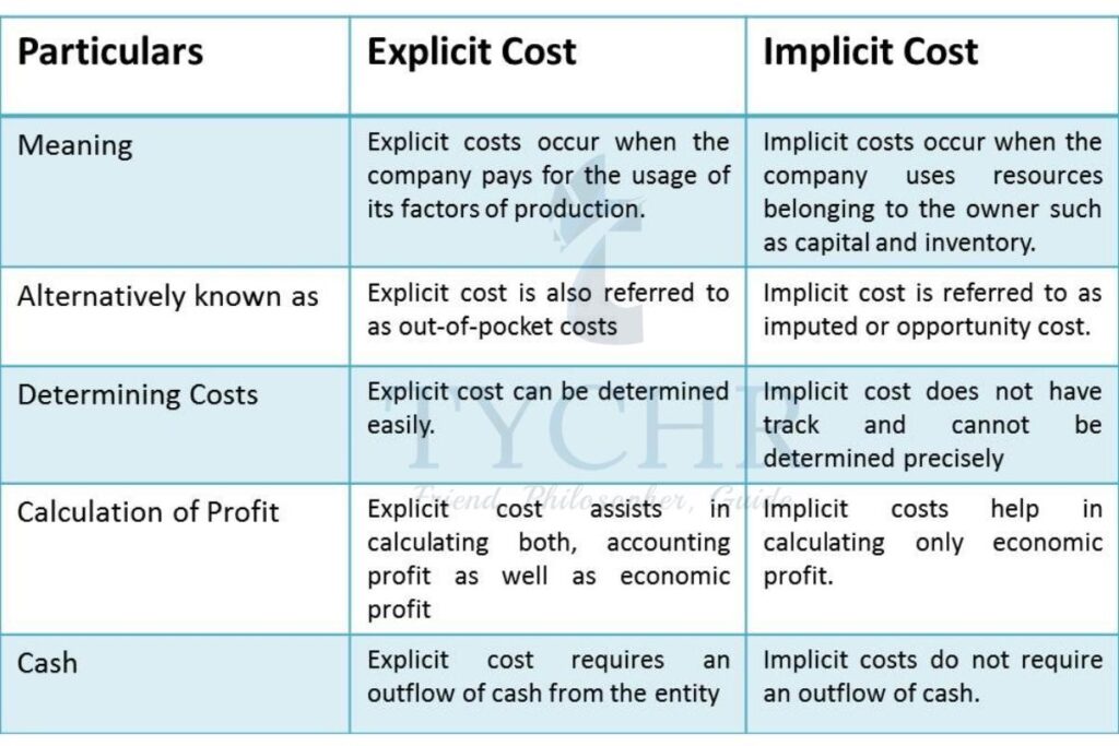
Economic Costs It is the sum of the explicit and implicit costs or total opportunity costs incurred by a firm for its use of resources, whether purchased or self owned. When economists refer to ‘costs’ they mean ‘economic costs’.
Cost of Production in the short run
Fixed, variable and total costs in the short run and long run:
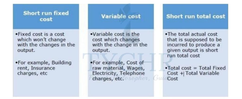
Note: In the short run, the firm’s TC= TFC + TVC. But in the long run, there are no fixed costs, therefore a firm’s total cost = variable costs.
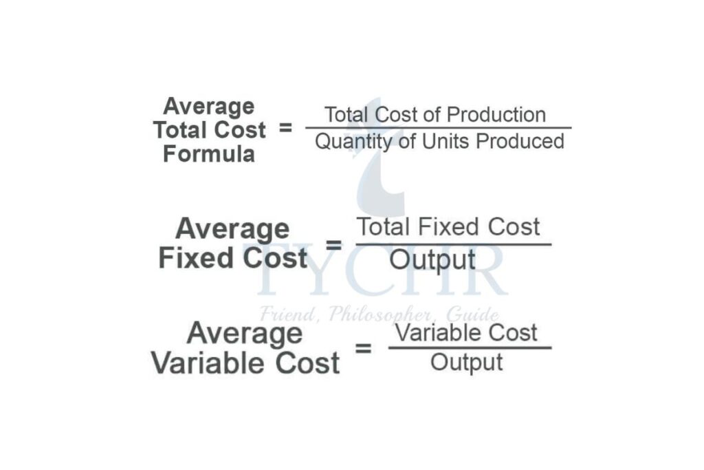
Average and Marginal costs
Cost curves and product curves
Short run cost curves:
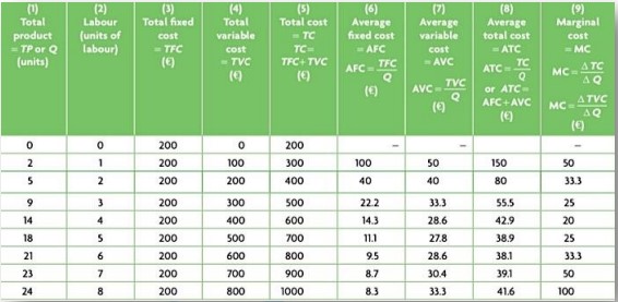
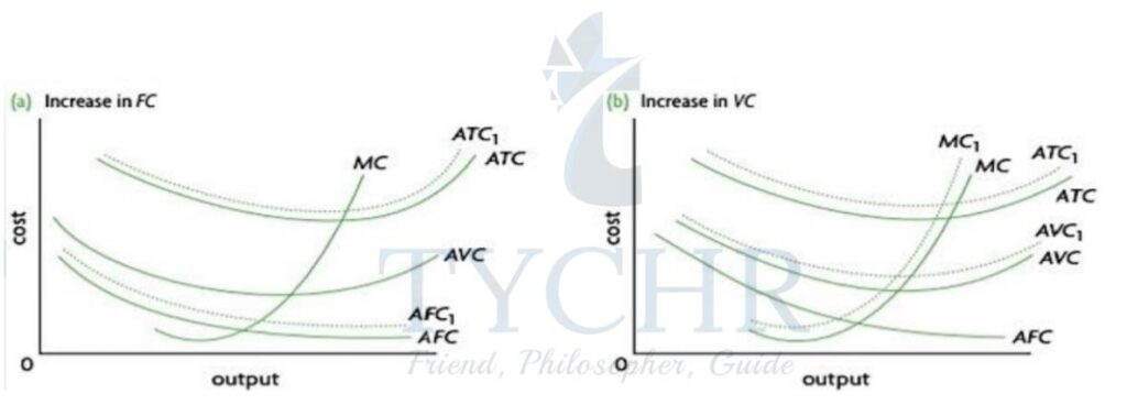
Fig (a)
- The TFC curve is II to x-axis, indicating that it doesn’t change with output.
- TVC increases as output increases. But it doesn’t increase at a constant rate because of the law of diminishing returns.
- TC = TFC + TVC so the vertical difference is equal to TFC.
Fig (b)
AFC | AVC/ATC/MC |
Falls at output increase because of fixed costs divided by increased output. | First falls, reach minimum and then they rise. ATC = AFC + AFC vertical difference = AFC. |
Relationship between Cost and Product curves
Note: Product curves are mirror images of the cost curve.
When the additional output produced by an extra worker is the most it can be, then the extra labour cost of producing an additional unit of output is the least it can be.
Note: The ‘U’ shape of AVC, ATC and MC curves is due to the law of diminishing returns.
Shifts in the cost curves
Change in resource prices or a change in technology changes the cost curves. If both increase – high cost of production – will shift TFC, TC, AFC, ATC curve upwards.
Variable and marginal costs unaffected.
Cost of Production in the long run :
In the long run, there are no fixed factors, all are variable inputs. Let’s see what happens to output when firm changes all it’s inputs.
There are 3 possibilities
- Constant returns to scale
Output increases in the same proportion as all inputs.
% increase in output = % increase in input - Increasing returns to scale
% increase in output > % increase in all inputs. - Decreasing returns to scale
% increase in output < % increase in all inputs.
Long run ATC in relation to short run ATC curves
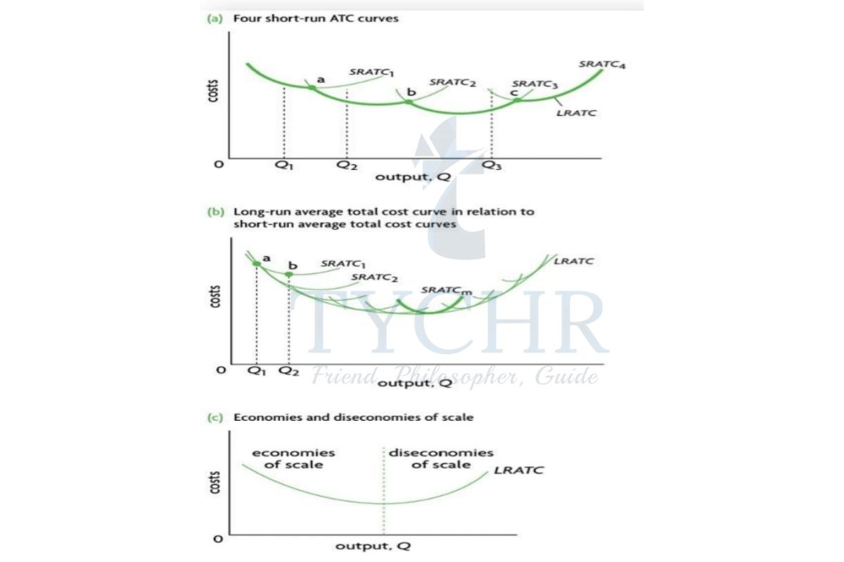
The long run ATC curves (LRATC) is defined as a curve that shows the lowest possible average cost that can be attained by a firm for any level of output, when all of the firm’s input are variable. It is a curve that just touches (is tangent to ) each of many short run average total cost curves. It is also known as a planning curve.
Shape of LRATC curve
The U shape of LRATC curve is due to economies and diseconomies of scale.
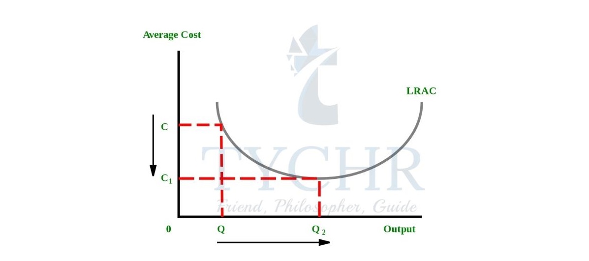
Economies of scale
Economies of scale are factors that lead to a reduction in average costs that are obtained by growth of a business. There are five economies of scale:
Purchasing economies: Larger capital means you get discounts when buying bulk.
Marketing: More money for advertising and own transportation, cutting costs.
Financial: Easier to borrow money from banks with lower interest rates.
Managerial: Larger businesses can now afford specialist managers in all departments, increasing efficiency.
Technical: They can now buy specialized and latest equipment to cut overall production costs.
Diseconomies of scale
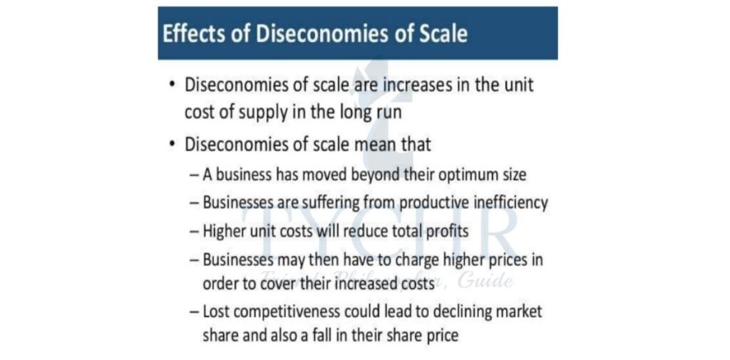
Note: Some studies suggests that after exhausting economies of scale, many firms exhibit constant
returns to scale, and do no run into diseconomies of scale even if the size becomes very large.
Revenue
Total revenue, Marginal revenue and Average revenue
Total Revenue (TR): The total earnings of a firm from sale of its output.
TR= P X Q
Marginal Revenue (MR): The additional revenue of a firm arising from the sale of an additional unit of output.
MR = change in TR / change in Q
Average Revenue (AR): Revenue per unit of output.
AR = TR / Q
Profits
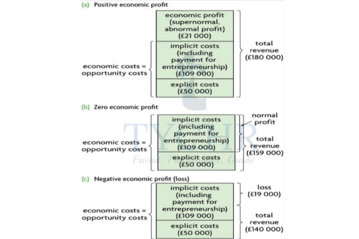
Economic profit = Total revenue minus economic costs ( or total opportunity costs or the sum of explicit plus implicit costs).
Normal profits = The minimum amount of revenue required by a firm so that it will be induced to keep running, which is that part of the revenue that covers implicit costs , including entrepreneurship (after all implicit costs have been covered). entrepreneurship (after all implicit costs have been covered).
Note: Why does a firm continue to operate even when earning zero economic profit?
When a firm is earning normal profit, it has covered all its opportunity cost (implicit cost) and will continue to operate.
Positive and Negative Economic Profit
Positive economic profit is also known as supernormal or abnormal profit. Note: Economic profit can be positive, negative or zero.
- Positive Economic Profit (supernormal profit) : TR > Economic profit.
- Zero Economic Profit (normal profit) : TR = Economic profit.
- Negative Economic Profit (loss) : TR < Economic profit.
Goals of Firms
Profit Maximization It involves determining the level of output that the firm should produce to make as large a profit as possible.
There are 2 approaches to analyze profit
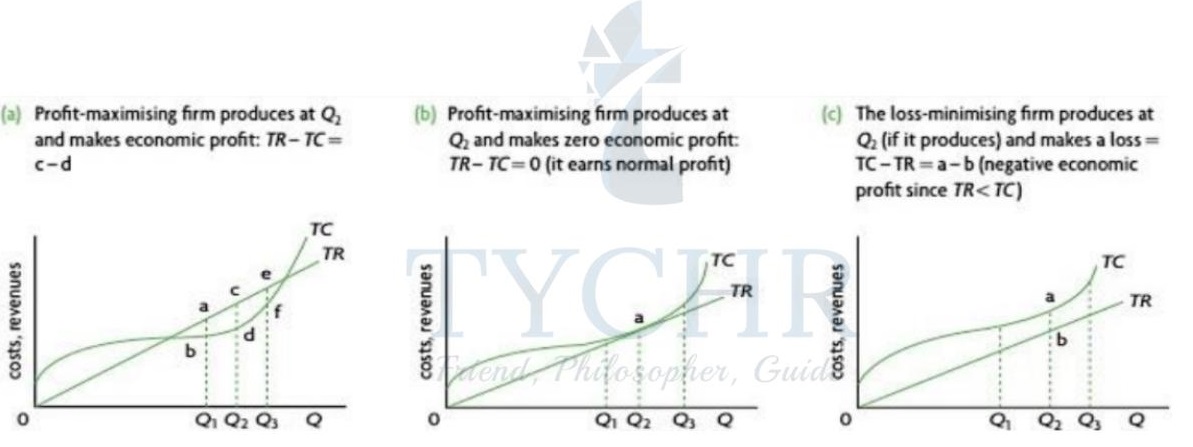
- TR – TC approach: Profit = TR – TC
The firm’s profit maximisation rule is to produce the level of output where TR – TC = Economic Profit. (economic profit is as large as possible)
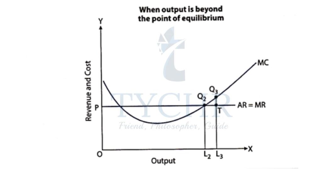
MR – MC approach:
Revenue Maximization Maximizing revenues by selling larger quantities of goods.
Growth Maximization A firm focuses on growth rather than profits. It can be attractive for the
Following reasons
Helps achieve economies of scale.
Helps in product diversification.
Greater market power.
Managerial Utility Maximisation In view of the principle that management is different from ownership, managers develop their own objectives to maximize their utility.
Managerial utility can be derived from Increased salaries, fringe benefits, etc.
Satisficing This can be referred to as a strategy that strives for satisfactory decision making. It is aimed at taking decisions that are okay enough to tackle a situation, but not the best possible situations.
Ethical and Environmental concerns
Corporate Social Responsibility : A firm focuses on environmental and ethical issues by taking up socially beneficial activities like –
- Non- polluting activities.
- Support for human rights.
- Donations.