By the end of this chapter you should be familiar with:

• Modelling all types of functions like quadratic, cubic, etc.
• Developing and fitting models
• Testing and reflecting upon models
• Using models

POLYNOMIAL FUNCTIONS

Linear models are used to describe situations where one quantity increases at a fixed rate relative to another quantity. Interpolations are predictions based on values within the range of known values of the independent variable. Extrapolations are predictions based on values outside the range of known values of the independent variable.

DEVELOPING AND TESTING A LINEAR MODEL

To develop a linear model we need to:

1. Identify the input and output values.
2. Convert the data to two coordinate pairs.
3. Find the slope.
4. Write the linear model.
5. Use the model to make a prediction by evaluating the function at a given x
6. Use the model to identify an xvalue that results in a given y

Let’s use a linear model to investigate a towns population

Example: A town’s population has been growing linearly. In 2004 the population was 6,200. By 2009 the population had grown to 8,100. Assume this trend continues.

1. Predict the population in 2013.
2. Identify the year in which the population will reach 15,000.

Solution: The two changing quantities are the population size and time. While we could use the actual year value as the input quantity, doing so tends to lead to very cumbersome equations because the y-intercept would correspond to the year 0, more than 2000 years ago.

We will define our input as the number of years since 2004:

• Input: t, years since 2004
• Output: P(t), the town’s population

To predict the population in 2013 (t = 9), we would first need an equation for the population. Likewise, to find when the population would reach 15,000, we would need to solve for the input that would provide an output of 15,000. To write an equation, we need the initial value and the rate of change, or slope.
To determine the rate of change, we will use the change in output per change in input.

m = ​change in output/​​change in input​​

The problem gives us two input-output pairs. Converting them to match our defined variables, the year 2004 would correspond to t = 0, giving the point (0,6200). Notice that through our clever choice of variable definition, we have “given” ourselves the y-intercept of the function. The year 2009 would correspond to t = 5, giving the point (5,8100).
The two coordinate pairs are (0,6200) and (5,8100).

m = (8100 – 6200)/5 = 380 people per year

We already know the y-intercept of the line, so we can immediately write the equation:

P(t) = 380t + 6200

To predict the population in 2013, we evaluate our function at t = 9.

P(9) = 380(9) + 6,200 = 9,620

If the trend continues, our model predicts a population of 9,620 in 2013.

To find when the population will reach 15,000, we can set P(t)=15000 and solve for t.

15000 = 380t + 6200 
8800 = 380t 
t = 23.158

Our model predicts the population will reach 15,000 in a little more than 23 years after 2004, or somewhere around the year 2027.

QUADRATIC MODELS

Recall a quadratic function in the standard form f(x) = ax² + bx + c, where a is the leading coefficient, b is the middle term coefficient, and c is the constant (y-intercept) of the function. Those three values can tell a lot about the behaviour of the function and the real-life scenario it models. You might also remember that a graph of a quadratic function is called a parabola.

Let’s start with the leading coefficient a that determines how curved the parabola is. If the a value is positive, the parabola opens up, and the function has a minimum. Similarly, if a < 0, the parabola opens down and the function will have a maximum. The minimum or the maximum value of a

quadratic function is also called the vertex (h,k), where h is the x-value of the vertex and k is the y-value of the vertex.

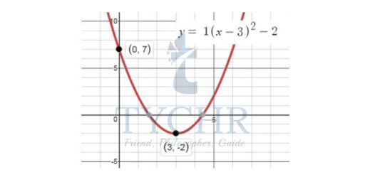
VERTEX FORM

Quadratic function using the vertex and the leading coefficient, and the resulting vertex form is f(x) = a(x – h)² + k. Pay attention to the signs in the vertex form. For example, if the vertex is at (-3,2) and a = 1, the equation would be f(x) = (x + 3)² + 2. However, if the vertex was at (3,-2), the signs in the equation would change and result in f(x) = (x – 3)² – 2.

FACTORED FORM

The last form of a quadratic function that can be used to model a real-world scenario is factored form f(x) = a (x – r₁)(x – r₂), where r₁ and r₂ are the zeros (x-intercepts) of the function. Remember that the factors need to be set equal to zero and solve for x to ‘see’ the actual x-intercept.

For example, if f(x) = (x – 2)(x + 3), then x – 2 = 0 and x = 2. Similarly, x + 3 = 0, thus x = -3.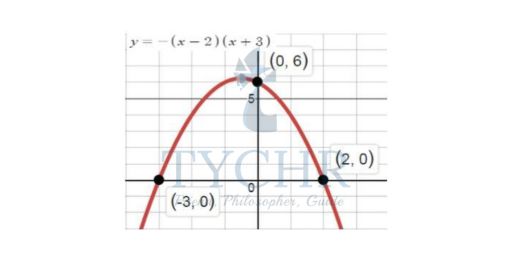Example: You just bought yourself a brand new soccer ball and you want to know how high you can kick it. You know you kicked the ball from the ground level, which is the y-intercept and first zero at the same time (0,0). You estimated that the ball hit the ground approximately 60 feet from where you kicked it (that will be the second x-intercept). Your friend estimated that when the ball was 5 feet away from you, it was about 10 feet up in the air (additional point on the graph, (5,10)).

Now let’s figure out the given: zeros: (0,0) and (0,60), and another point (5,10).
Form to use: factored form y = a(x – r₁)(x – r₂)
Substitute the zeros for the r₁ and r₂ and the other point for x and y.

Unknown: the vertex and the a value So we are going to have to solve for a in order to find the vertex.

As expected, the leading coefficient is negative, the ball will reach the maximum and hit the ground following a path of a parabola that opens down.

So now we can use the a value and the zeros to rewrite the factored form f(x) = -.036(x – 0)(x – 60) of the trajectory of the ball you kicked. We do not see the actual vertex in the factored form, but no fear, we have technology to help us out! Use any graphic calculator, handheld or online, to graph f(x) and find the highest y value either in the table or on a graph. Here is what you should see. The maximum height of the kick was approximately 32.4 feet.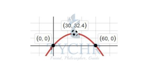

CUBIC MODELS

A Cubic Model uses cubic functions of the form ax³ + bx² + cx + d can be used to model real-world situations. They can be used to model three-dimensional objects to allow you to identify a missing dimension or explore the result of changes to one or more dimensions.

Example: Consider a situation in which a rectangular piece of cardboard is folded into a box. The folding is made possible by cutting squares out of the four corners of the cardboard.

Calculate the maximum volume possible of a box made from a sheet of cardboard 12″ x 8″.

The function v(x) = (12−2x)(8−2x)x could be used to represent the volume of the box as a function of x, the side-length of the squares cut out of the corners. If we multiply out the factors of this function we can verify that this is a cubic function:

v(x) = (12−2x)(8−2x)x = 4x³ − 40x² + 96x

This function could be used to find the maximum possible volume of the box. We can also analyse the graph to understand how the volume changes as a function of x.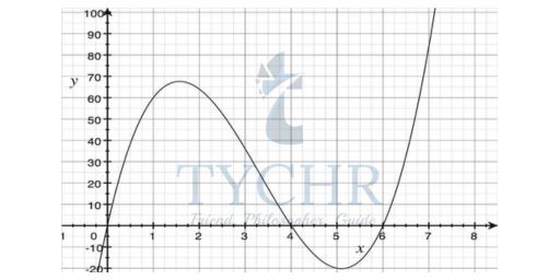

When analysing the function to determine the maximum volume of the box, we only look at the portion of the graph that looks “parabolic”. This is because the function ceases to model the situation if x is more than 4. If we cut out {4×4} squares, we would cut out the entire short side of the cardboard rectangle, and we would not be able to make a box. Focusing then on the interval (0, 4) we can see that the volume of the box increases, and then decreases.

If we are using a graphing calculator and want to know the volume of a box with particular dimensions, we can trace on the graph, input values into the table, or take advantage of the graph being in trace mode. That is, if you press GRAPH to view the graph, and then press TRACE, you can input x values. For example, say that you wanted to cut out squares of side-length 2.5. Press TRACE, then press 2.5, then press ENTER. At the bottom of the screen you will see x = 2.5 and y = 52.5. This tells you that the volume of the box will be 52.5in³.

EXPONENTIAL AND LOGARITHMIC MODELS

Exponential model arise in situations where the rate of change is a constant factor.

EXPONENTIAL GROWTH

Function

y = C e^kt, k > 0

Features

• Asymptotic to y = 0 to left
• Passes through (0,C)
• C is the initial value
• Increases without bound to right

Some of the things that exponential growth is used to model include population growth, bacterial growth, and compound interest.

To be given the initial value, that is the value when x = 0, then you already know the value of the constant C. The only thing necessary to complete the model is to have one additional point on the graph. Plug in the values for x, y, and C, and solve for k.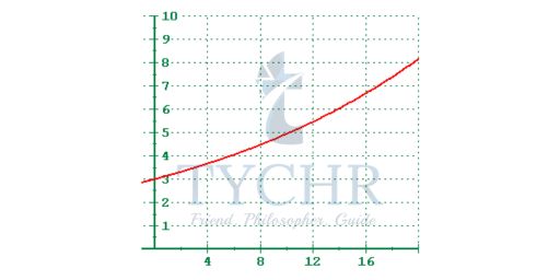

EXPONENTIAL DECAY (decreasing form):

Function

y = C e^-kt, k > 0

Features

• Asymptotic to y = 0 to right
• Passes through (0,C)
• C is the initial value
• Decreasing, but bounded below by y=0

Exponential decay and be used to model radioactive decay and depreciation.

Exponential decay models decrease very rapidly, and then level off to become asymptotic towards the x-axis.

Like the exponential growth model, if you know the initial value then the rest of the model is fairly easy to complete.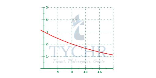

EXPONENTIAL DECAY (increasing form):

Function

y = C(1 – e^-kt), k > 0

Features

• Asymptotic to y = C to right
• Passes through (0,0)
• C is the upper limit
• Increasing, but bounded above by y=C

Exponential decay models of this form can model sales or learning curves where there is an upper limit. This is done by subtracting the exponential expression from one and multiplying by the upper limit.

Exponential decay models of this form will increase very rapidly at first, and then level off to become asymptotic to the upper limit.

Like the other exponential models, if you know upper limit, then the rest of the model is fairly easy to complete.

The calculator will not fit the increasing model involving exponential decay directly.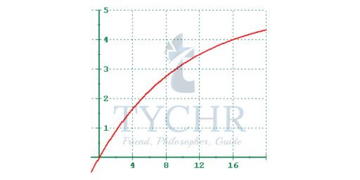

LOGARITHMIC MODEL

Function

y = a + b ln x

Features

• Increases without bound to right
• Passes through (1,a),
• Very rapid growth, followed by slower growth,
• Common log will grow slower than natural log
• b controls the rate of growth

The logarithmic model has a period of rapid increase, followed by a period where the growth slows, but the growth continues to increase without bound. This makes the model inappropriate where there needs to be an upper bound. The main difference between this model and the exponential growth model is that the exponential growth model begins slowly and then increases very rapidly as time increases.

Several physical applications have logarithmic models. The magnitude of earthquakes, the intensity of sound, the acidity of a solution.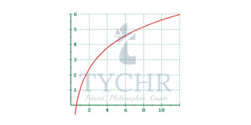

Example: How long will it take for 10% of a 1000-gram sample of uranium-235 to decay?

Solution:

y = 1000eln(0.5)t/703,800,000
900 = 1000 𝑒^{1000eln(0.5)t/703,800,000}
ln(0.9) = ln(0.5)t/703,800,000
t = 106,979,777 years

TRIGONOMETRIC MODELS

Any motion that repeats itself in a fixed time period is considered periodic motion and can be modelled by a sinusoidal function. The amplitude of a sinusoidal function is the distance from the midline to the maximum value, or from the midline to the minimum value. The midline is the average value. Sinusoidal functions oscillate above and below the midline, are periodic, and repeat values in set cycles.

sin(x±2πk) = sinx and cos(x±2πk) = cosx
The general forms of a sinusoidal equation are given as

y = Asin(Bt−C) + D
or
y = Acos(Bt−C)+ D
where amplitude=|A|, B is related to period such that the period = 2π/B, C is the phase shift such that C/B denotes the horizontal shift, and D represents the vertical shift from the graphs parent graph.

Note that the models are sometimes written as

y = Asin(ωt±C) + D
or
y = Acos(ωt±C) + D

with a period that is given as 2π/ω.
The difference between the sine and the cosine graphs is that the sine graph begins with the average value of the function and the cosine graph begins with the maximum or minimum value of the function.

Example: The hour hand of the large clock on the wall in Union Station measures 24 inches in length. At noon, the tip of the hour hand is 30 inches from the ceiling. At 3 PM, the tip is 54 inches from the ceiling, and at 6 PM, 78 inches. At 9 PM, it is again 54 inches from the ceiling, and at midnight, the tip of the hour hand returns to its original position 30 inches from the ceiling. Let y equal the distance from the tip of the hour hand to the ceiling x hours after noon. Find the equation that models the motion of the clock and sketch the graph.

Solution:

To model an equation, we first need to find the amplitude.

|A|=|(78 − 30)/2| = 24

The clock’s cycle repeats every 12 hours. Thus,

B = 2π/12 = π/6

The vertical shift is

D = (78+30)/2 = 54

There is no horizontal shift, so C=0. Since the function begins with the minimum value of y when x=0 (as opposed to the maximum value), we will use the cosine function with the negative value for A. In the form y = Acos(Bx±C) + D, the equation is:

y = −24cos(πx/6) + 54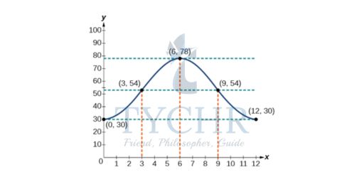

LOGISTIC MODELS

Function

y = a / (1 + b e^-kx ), k > 0

Features

• Asymptotic to y = a to right,
• Asymptotic to y = 0 to left,
• Passes through (0, a/(1+b))
• Slow growth, followed by moderate growth, followed by slow growth

The logistics model begins with a slow growth, followed by a period of moderate growth, and then back to a period of slow growth. It has an upper limit that cannot be exceeded.

The Logistics model can be used to approximate sales and advertising or population growth where there is not the capacity for unlimited growth.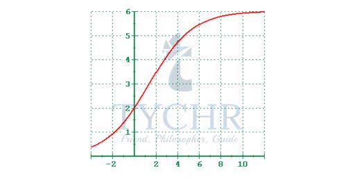

Example: In a class of 30 students, one student comes sick to school one day the infection of the remaining students follows a logistic model of the form S(d) = L / (1 + Ce^-kd ) where d is the number of days since the initial infection.

1. Write down the value of L
2. Find the value of C given that the first student is sick on day 0
3. Given that half the students are infected after 5 days, find the value of k
4. Sketch a graph

Solution:

1. Since the maximum number of students infected = 30, L = 30
2. S(0) = 1 S(0) = 30 / (1 + Ce^{-k x 0} ) C = 29
3. The point of infection is (5,15). Hence, lnC/k = 5 ln29/5 = k k = 0.673
4.  

DIRECT AND INVERSE VARIATION

Direct variation describes a simple relationship between two variables. We say y varies directly with x if:

y = kx

for some constant k.
This means that as x increases, y increases and as x decreases, y decreases and that the ratio between them always stays the same.

The graph of the direct variation equation is a straight line through the origin.

Direct variation models are simplified models of the form y = axⁿ for n > 0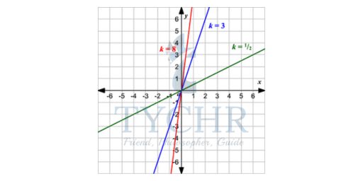
Inverse variation describes another kind of relationship. We say y varies inversely with x if:

xy = k

for some constant k.

This means that as x increases, y decreases and as x decreases, y increases.

The graph of the inverse variation equation is a hyperbola.

Inverse variation models are simplified models of the form yxⁿ = a for n > 0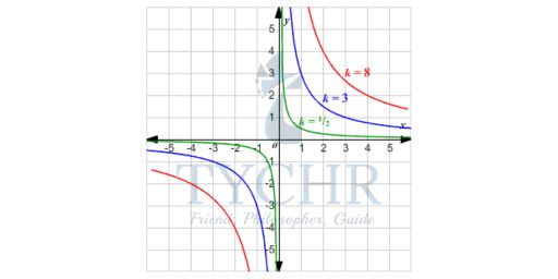
Example: The cost C of a phone call varies directly with the call m in minutes. A recent 5-minute phone call cost $0.60

1. Formulate a direct variation model
2. Find the length of the call that costs $1.56

Solution:

1. Since a 5- minute phone call costs $0.60, we have C = am 60 = a(5) a = 0.12
2. C = am 56 = m(0.12) m = 13 minutes

CHOOSING A MODEL

1. If it’s a constant, try a linear model.
2. If the quantity is increasing/decreasing by a fixed percentage or ratio, try an exponential model.
3. If the quantity is increasing/decreasing at a linearly increasing/decreasing rate, try a quadratic model.
4. If it relates to the volume of a linear quantity, try a cubic model.
5. If it’s cyclic/periodic/repeating, try a trigonometric model.