By the end of this chapter you should be familiar with:

• Contingency tables
• Observed frequencies and expected frequencies
• Null hypothesis and alternative hypothesis
• Significance level
• Degrees of freedom
• Probability values
• χ2 test for independence and goodness of fit
• t-test
• Spearman’s rank correlation

SPEARMAN’S RANK CORRELATION COEFFICIENT

Contingency tables (also called crosstabs or two-way tables) are used in statistics to summarize the relationship between several categorical variables. A contingency table is a special type of frequency distribution table, where two variables are shown simultaneously.

The Spearman’s Rank Correlation Coefficient is used to discover the strength of a link between two sets of data. The notation used is r_s.

Spearman’s correlation coefficient shows the extent to which one variable increases or decreases as the other variable increases. Such behaviour is described as ‘monotonic’.

A value of 1 means the set of data is strictly increasing, a value of -1 means the set of data is strictly decreasing and a value of 0 means no monotonic behaviour.

Spearman’s rank correlation coefficient is calculated from a sample of N data pairs (X, Y) by first creating a variable U as the ranks of X and a variable V as the ranks of Y (ties replaced with average ranks). Spearman’s correlation is then calculated from U and V using: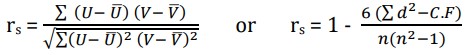Example: Find the Spearman’s rank correlation coefficient for the following data:

Solution: Make a table: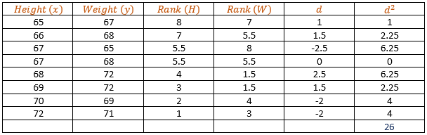

Where d = H – W

CF₁​ = 2(4 − 1)/12 ​= (2 × 3)/12 ​= 0.5 CF₂ ​= (2 × 3)/12 ​= 0.5

C.F = ∑d²+ CF₁ ​+ CF₂ ​= 26 + 0.5 + 0.5 = 27

 r_s = 1 – (6 × 27)/ (8×6) ​= 0.679

HYPOTHESIS TESTING

A statistical hypothesis is an assumption about a population parameter. This assumption may or may not be true. Hypothesis testing refers to the formal procedures used by statisticians to accept or reject statistical hypotheses.

There are two types:

• Null hypothesis. The null hypothesis, denoted by H_o, is usually the hypothesis that sample observations result purely from chance.

• Alternative hypothesis. The alternative hypothesis, denoted by H₁ or H_a, is the hypothesis that sample observations are influenced by some non-random cause.

Statisticians follow a formal process to determine whether to reject a null hypothesis, based on sample data. This process, called hypothesis testing, consists of four steps.

• State the hypotheses. This involves stating the null and alternative hypotheses. The hypotheses are stated in such a way that they are mutually exclusive. That is, if one is true, the other must be false.
• Formulate an analysis plan. The analysis plan describes how to use sample data to evaluate the null hypothesis. The evaluation often focuses around a single test statistic.
• Analyse sample data. Find the value of the test statistic (mean score, proportion, t statistic, z-score, etc.) described in the analysis plan.
• Interpret results. Apply the decision rule described in the analysis plan. If the value of the test statistic is unlikely, based on the null hypothesis, reject the null hypothesis.

A test of a statistical hypothesis, where the region of rejection is on only one side of the sampling distribution, is called a one-tailed test and a test of a statistical hypothesis, where the region of rejection is on both sides of the sampling distribution, is called a two-tailed test.

TEST FOR A BINOMIAL PROBABILITY

To hypothesis test with the binomial distribution, we must calculate the probability, p, of the observed event and any more extreme event happening. We compare this to the level of significance α. If p > α then we do not reject the null hypothesis. If p < α we accept the alternative hypothesis.

Example: A coin is tossed twenty times, landing on heads six times. Perform a hypothesis test at a 5% significance level to see if the coin is biased.

Solution: First, we need to write down the null and alternative hypotheses. In this case
H₀: The coin is not biased.
H₁: The coin is biased in favour of tails.

The important thing to note here is that we only need a one-tailed test as the alternative hypothesis says “in favour of tails”. A two-tailed test would be the result of an alternative hypothesis saying “The coin is biased”.

P[X ≤ 6] = 0.058
P[X ≤ 5] = 0.021

We would have had to reject the null hypothesis and accept the alternative hypothesis. So the point at which we switch from accepting the null hypothesis to rejecting it is when we obtain 5 heads. This means that 5 is the critical value.

TEST FOR A POISSON DISTRIBUTION

Testing hypotheses with the Poisson distribution is very similar to testing them with the binomial distribution. If the probability is greater than α, the level of significance, then the null hypothesis is accepted. If it is less than α, we accepted the alternative hypothesis.

Example: An existing make of car is known to break down on average one and a half times per year. A new model is introduced and the manufacturer claims that this model is less likely to break down. Ten

randomly selected cars break down a total of eight times within the first year. Test the manufacturer’s claim at a 5% significance level.

Solution: Let X be the number of break downs of the new model of car in a year. Since we have an average rate and the data is discrete, we need to use a Poisson distribution. So X ∼ Poisson(λ) with λ=1.5. The null and alternative hypotheses will be

H₀ : H₁ : λ = 1.5, λ < 1.5

We need to decide whether P[X ≤ 8] < α, where α=0.05 is the significance level. Firstly, the expected number of breakdowns λ_t = 1.5×10 = 15.
We use the cumulative tables with λ_t = 15 and x=8 to see P[X ≤ 8] = 0.0374
P[X ≤ 8] = 0.0374 < 0.05 = α

So we accept the alternative hypothesis. The average rate of breakdowns has decreased.

TEST FOR A NORMAL DISTRIBUTION

When constructing a confidence interval with the standard normal distribution, these are the most important values that will be needed.

These values are obtained from the inverse of the cumulative distribution function of the standard normal distribution. i.e. we need to consider ∅^-1x. For example, when we look for the probability, say, that z < 2.33, we get P[z < 2.33] = 0.99. Now if we have a 1% significance level, we need a 99% confidence interval so we need z distribution of sample means where μ is the true mean and μ₀ is the current accepted population mean. Draw samples of size n from the population. When n is large

enough and the null hypothesis is true the sample means often follow a normal distribution with mean μ₀ and standard deviation 𝜎/√𝑛 . This is called the distribution of sample means and can be denoted by 𝑥̅ ∼ N(μ₀, 𝜎/√𝑛). This follows from the central limit theorem.

The z-score will this time be obtained with the formula

z = 𝑥̅− 𝜇₀/𝜎/√𝑛
So if μ = 𝜇₀, X ∼ N(𝜇₀, 𝜎/√𝑛) and z ∼ N(0, 1)

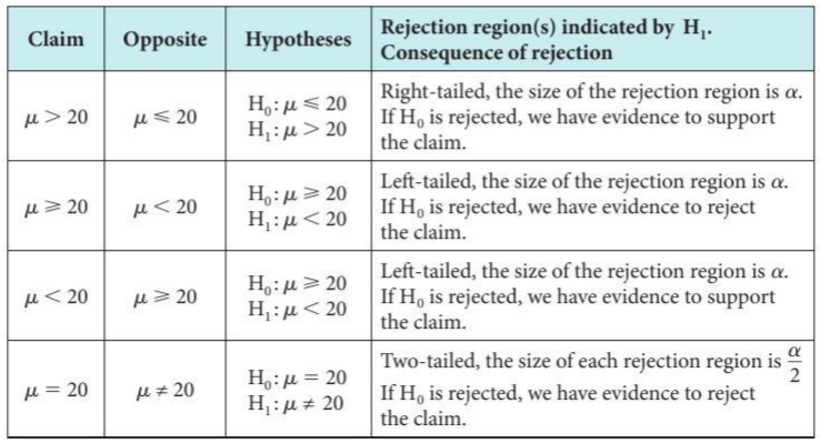
The alternative hypothesis will then take one of the following forms: depending on what we are testing.

Example: An automobile company is looking for fuel additives that might increase gas mileage. Without additives, their cars are known to average 25 mpg (miles per gallons) with a standard deviation of 2.4 mpg on a road trip from London to Edinburgh. The company now asks whether a particular new additive increases this value. In a study, thirty cars are sent on a road trip from London to Edinburgh. Suppose it turns out that the thirty cars averaged 𝑥̅ = 25.5 mpg with the additive. Can we conclude from this result that the additive is effective?

Solution: We are asked to show if the new additive increases the mean miles per gallon. The current mean μ=25 so the null hypothesis will be that nothing changes. The alternative hypothesis will be that μ>25 because this is what we have been asked to test.

H₀: μ = 25 H₁: μ > 25

Now we need to calculate the test statistic. We start with the assumption the normal distribution is still valid. This is because the null hypothesis states there is no change in μ. Thus, as the value σ=2.4 mpg is known, we perform a hypothesis test with the standard normal distribution. So the test statistic will be a z score. We compute the z score using the formula

z = (𝑥̅− 𝜇₀)/𝜎/√𝑛 = (25.5−25)/2.4/√30

We are using a 5% significance level and a (right-sided) one-tailed test, so α=0.05 so from the tables we obtain z_1- α= 1.645 is our test statistic.

As 1.14 < 1.645, the test statistic is not in the critical region so we cannot reject H₀. Thus, the observed sample mean 𝑥̅ is consistent with the hypothesis H₀: μ = 25 on a 5% significance level.

THE T-TEST

The t-test is a statistical test which is widely used to compare the mean of two groups of samples. It is therefore to evaluate whether the means of the two sets of data are statistically significantly different from each other.

There are many types of t test:

1. The one-sample t-test, used to compare the mean of a population with a theoretical value.
2. The unpaired two sample t-test, used to compare the mean of two independent samples.
3. The paired t-test, used to compare the means between two related groups of samples.

ONE SAMPLE T-TEST

As mentioned above, one-sample t-test is used to compare the mean of a population to a specified theoretical mean (μ).

Let X represents a set of values with size n, with mean m and with standard deviation S. The comparison of the observed mean (m) of the population to a theoretical value μ is performed with the formula below:

t = (m−μ)/ 𝑠/√𝑛

To evaluate whether the difference is statistically significant, you first have to read in t test table the critical value of Student’s t distribution corresponding to the significance level alpha of your choice (5%). The degrees of freedom (df) used in this test are:

df = n−1

TWO SAMPLE T-TEST

Independent (or unpaired two sample) t-test is used to compare the means of two unrelated groups of samples.

• Let A and B represent the two groups to compare.
• Let m_Aand m_B represent the means of groups A and B, respectively.
• Let n_Aand n_B represent the sizes of group A and B, respectively.

The t test statistic value to test whether the means are different can be calculated as follows: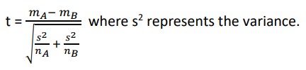Once t-test statistic value is determined, you have to read in t-test table the critical value of Student’s t distribution corresponding to the significance level alpha of your choice (5%). The degrees of freedom (df) used in this test are:

df = n_A + n_B – 2

PAIRED SAMPLE T-TEST

To compare the means of the two paired sets of data, the differences between all pairs must be, first, calculated.

Let d represents the differences between all pairs. The average of the difference d is compared to 0. If there is any significant difference between the two pairs of samples, then the mean of d is expected to be far from 0.

The t-test statistic value can be calculated as follows:

t = m/𝑠√n

where m and s are the mean and the standard deviation of the difference (d), respectively. n is the size of d.

Once t value is determined, you have to read in t-test table the critical value of Student’s t distribution corresponding to the significance level alpha of your choice (5%). The degrees of freedom (df) used in this test are:

df = n – 1

Example: Find the t-test value for the following two sets of values: 7, 2, 9, 8 and 1, 2, 3, 4?

Solution:

Mean for the first set of data = (7+2+9+8)/4 = 6.5

Standard deviation for the first set of data = 3.11

Mean for the first set of data = (1+2+3+4)/4 = 2.5

Standard deviation for the first set of data = 1.29

For t-test value: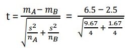   t = 2.36

CHI-SQUARED TEST FOR INDEPENDENCE

A chi-square test for independence is applied when you have two categorical variables from a single population. It is used to determine whether there is a significant association between the two variables.

Degrees of freedom. The degrees of freedom (df) is equal to:

df = (r – 1) (c – 1)

where r is the number of levels for one categorical variable, and c is the number of levels for the other categorical variable.

The test statistic is a chi-square random variable (Χ²) defined by the following equation.

X² = ∑ (𝑓₀ − 𝑓_𝑐)² /𝑓𝑐

Where f₀ are the observed values and f_c are the expected values.

As we already know, that if this number is larger than a critical value then we reject null hypothesis.

The p-value is the probability of observing a sample statistic as extreme as the test statistic. Since the test statistic is a chi-square, use the chi-square distribution calculator to assess the probability associated with the test statistic. Use the degrees of freedom computed above.

Example: A public opinion poll surveyed a simple random sample of 1000 voters. Respondents were classified by gender (male or female) and by voting preference (Republican, Democrat, or Independent). Results are shown in the contingency table below.

Is there a gender gap? Do the men’s voting preferences differ significantly from the women’s preferences? Use a 0.05 level of significance.

Solution:

The solution to this problem takes four steps: (1) state the hypotheses, (2) formulate an analysis plan, (3) analyse sample data, and (4) interpret results. We work through those steps below:

• State the hypotheses. The first step is to state the null hypothesis and an alternative hypothesis.
  H_o: Gender and voting preferences are independent.
  H_a: Gender and voting preferences are not independent.
• Formulate an analysis plan. For this analysis, the significance level is 0.05. Using sample data, we will conduct a chi-square test for independence.
• Analyse sample data. Applying the chi-square test for independence to sample data, we compute the degrees of freedom, the expected frequency counts, and the chi-square test statistic. Based on the chi-square statistic and the degrees of freedom, we determine the p-value.
  DF = (r – 1) (c – 1) = (2 – 1) (3 – 1) = 2
  f_1,1 = (400 450) / 1000 = 180000/1000 = 180
  f_1,2 = (400 450) / 1000 = 180000/1000 = 180
  f_1,3 = (400 100) / 1000 = 40000/1000 = 40
  f_2,1 = (600 450) / 1000 = 270000/1000 = 270
  f_2,2 = (600 450) / 1000 = 270000/1000 = 270
  f_2,3 = (600 100) / 1000 = 60000/1000 = 60
  X² = ∑ (𝑓₀ − 𝑓_𝑐)² /𝑓𝑐
  Χ² = (200 – 180)²/180 + (150 – 180)²/180 + (50 – 40)²/40 + (250 – 270)²/270 + (300 – 270)²/270 + (50 – 60)²/60
  Χ² = 400/180 + 900/180 + 100/40 + 400/270 + 900/270 + 100/60
  Χ² = 2.22 + 5.00 + 2.50 + 1.48 + 3.33 + 1.67 = 16.2
  P(X² > 16.2) = 0.0003

Since the P-value (0.0003) is less than the significance level (0.05), we cannot accept the null hypothesis. Thus, we conclude that there is a relationship between gender and voting preference.

CHI-SQUARED GOODNESS OF FIT-TEST

A chi-square goodness of fit test is applied when you have one categorical variable from a single population. It is used to determine whether sample data are consistent with a hypothesized distribution.

We follow the same steps followed for chi-square test for independence but here

• Degrees of freedom. The degrees of freedom (DF) is equal to the number of levels (k) of the categorical variable minus 1.
  DF = k – 1
• Expected frequency counts. The expected frequency counts at each level of the categorical variable are equal to the sample size times the hypothesized proportion from the null hypothesis
  E_i = np_i
  where E_i is the expected frequency count for the ith level of the categorical variable, n is the total sample size, and p_i is the hypothesized proportion of observations in level i.
• Test statistic. The test statistic is a chi-square random variable (Χ²) defined by the following equation.
  Χ² = Σ [ (O_i – E_i)² / E_i ]
  where O_i is the observed frequency count for the ith level of the categorical variable, and E_i is the expected frequency count for the ith level of the categorical variable.

Example: Acme Toy Company prints baseball cards. The company claims that 30% of the cards are rookies, 60% veterans but not All-Stars, and 10% are veteran All-Stars. Suppose a random sample of 100 cards has 50 rookies, 45 veterans, and 5 All-Stars. Is this consistent with Acme’s claim? Use a 0.05 level of significance.

Solution: The solution to this problem takes four steps: (1) state the hypotheses, (2) formulate an analysis plan, (3) analyse sample data, and (4) interpret results. We work through those steps below:

• State the hypotheses. The first step is to state the null hypothesis and an alternative hypothesis.

• • Null hypothesis: The proportion of rookies, veterans, and All-Stars is 30%, 60% and 10%, respectively.
  • Alternative hypothesis: At least one of the proportions in the null hypothesis is false.
• Formulate an analysis plan. For this analysis, the significance level is 0.05. Using sample data, we will conduct a chi-square goodness of fit-test of the null hypothesis.
• Analyse sample data. We compute the degrees of freedom, the expected frequency counts, and the chi-square test statistic. Based on the chi-square statistic and the degrees of freedom, we determine the p-value.
  DF = k – 1 = 3 – 1 = 2 (E_i) = n x p_i
  (E₁) = 100 0.30 = 30
  (E₂) = 100 0.60 = 60
  (E₃) = 100 0.10 = 10
  Χ² = Σ [ (O_i – E_i)² / E_i ]
  Χ² = [ (50 – 30)² / 30 ] + [ (45 – 60)² / 60 ] + [ (5 – 10)² / 10 ]
  Χ² = (400 / 30) + (225 / 60) + (25 / 10) = 13.33 + 3.75 + 2.50 = 19.58
  The P-value is the probability that a chi-square statistic having 2 degrees of freedom is more extreme than 19.58.

We use the chi-square distribution calculator to find P(Χ² > 19.58) = 0.0001. Since the P-value (0.0001) is less than the significance level (0.05), we cannot accept the null hypothesis.

DECISION ERRORS

Two types of errors can result from a hypothesis test.

• Type I error. A Type I error occurs when the researcher rejects a null hypothesis when it is true. The probability of committing a Type I error is called the significance level. This probability is also called alpha, and is often denoted by α.
• Type II error. A Type II error occurs when the researcher fails to reject a null hypothesis that is false. The probability of committing a Type II error is called Beta, and is often denoted by β. The probability of not committing a Type II error is called the Power of the test.

The probability of not committing a type II error is called the power of a hypothesis test.

To compute the power of the test, one offers an alternative view about the “true” value of the population parameter, assuming that the null hypothesis is false. The effect size is the difference between the true value and the value specified in the null hypothesis.

Effect size = True value – Hypothesized value

The power of a hypothesis test is affected by three factors.

1. Sample size (n). Other things being equal, the greater the sample size, the greater the power of the test.
2. Significance level (α). The lower the significance level, the lower the power of the test. If you reduce the significance level (e.g., from 0.05 to 0.01), the region of acceptance gets bigger. As a result, you are less likely to reject the null hypothesis. This means you are less likely to reject the null hypothesis when it is false, so you are more likely to make a Type II error. In short, the power of the test is reduced when you reduce the significance level; and vice versa.
3. The “true” value of the parameter being tested. The greater the difference between the “true” value of a parameter and the value specified in the null hypothesis, the greater the power of the test. That is, the greater the effect size, the greater the power of the test.

Example: A machine fills milk bottles, the mean amount of milk in each bottle is supposed to be 32 Oz with a standard deviation of 0.06 Oz. Suppose the mean amount of milk is approximately normally distributed. To check if the machine is operating properly, 36 filled bottles will be chosen at random and the mean amount will be determined.

1. If an α = 0.05 test is used to decide whether the machine is working properly, what should the rejection criterion be?
2. Find the power of the test if the true mean takes on the following values: 31.97, 31.99, 32, 32.01, 32.03. Draw the power curve.
3. Find the probability of a type II error when the true mean is 32.03.

Solution:

1. X ∼ N(µ, σ² ), σ² = 0.062 , so ∼ N(µ, σ²/36).
   H₀: µ = 32, H_A: µ 6= 32,
   α = 0.05 = P( ≥ 32 + a) + P( ≤ 32 − a)
   = 2P((𝑋̅ − 32)/(σ/6) ≥ 𝑎 /(σ/6) ) = 2P(z ≥ 6a/σ )
   Therefore, 6a/σ = z = 1, 96, a = 0.0196. Hence the rejection regions are 32 ± a = 32.0196, 31.9804.
2. Power₁ = P(> 32.0196 | µ = 31.97) + P( < 31.9804 | µ = 31.97) = 0.8508
   Power₂ = P(z > 2.96) + P(z < −0.96) = 0.1700
   Power₃ = P(z > 1.96) + P(z < −1.96) = 0.05
   Power₄ = P(z > 0.96) + P(z < −2.96) = 0.1700
   Power₅ = P(z > −1.04) + P(z < −4.96) = 0.8508
3. β = 1 – Power₅ = 0.1492